# Colab environment cell
try:
    import pymrm  # noqa: F401
except ImportError:
    %pip install -q pymrm

import sys, os, time
if not os.path.exists("gallery_utils.py"):
    for p in ("../../shared", "../../../shared", "../shared"):
        if os.path.isdir(p):
            sys.path.insert(0, os.path.abspath(p))
            break
    else:
        import urllib.request
        urllib.request.urlretrieve(
            "https://raw.githubusercontent.com/computational-chemical-engineering/"
            "pymrm-gallery/main/shared/gallery_utils.py", "gallery_utils.py")

_T_START = time.time()
import numpy as np
import pandas as pd
import matplotlib.pyplot as plt
from IPython.display import HTML, Markdown, display

np.random.seed(19660501)   # nothing here is stochastic; seeded for reproducibility
PAGE = "A4.5-fuller-schettler-giddings"
pd.set_option("display.width", 120)

# DETERMINISM: a pandas Styler's text/plain repr carries a MEMORY ADDRESS and its
# HTML carries a RANDOM CSS id, so displaying one directly would make two runs of
# this notebook differ even with no other change. Route styled tables through
# HTML(...to_html()) with a pinned uuid, never display a Styler directly.
def show(styler):
display(HTML(styler.to_html()))Fuller-Schettler-Giddings: a correlation and the difference between fitting and predicting
sec:A
struct:S3
tier:T0
data:tier5
phase:gas
The most-used estimate of binary gas diffusivity, rebuilt from its own printed tables. Its famous 4.3 % is a goodness of fit to the 340 measurements the diffusion volumes were fitted to; held out one compound at a time, the same scheme gives 6.6 %.
Fuller-Schettler-Giddings binary gas diffusivities
Catalog ID: A4.5 · Structure: S3 (scalar diffusion) · Tier: T0
\[ D_{AB} \;=\; \frac{1.00\times10^{-3}\,T^{1.75}\,(1/M_A + 1/M_B)^{1/2}} {p\left[(\Sigma_A v_i)^{1/3} + (\Sigma_B v_i)^{1/3}\right]^{2}} \]
Two numbers, a temperature and a table of “diffusion volumes”, and you have a binary gas diffusivity to about five per cent. It is the estimate that ended up in every process simulator and every transport textbook, and it is sixty years old.
The number quoted for it is 4.3 %. This page establishes what that number is. Fuller, Schettler and Giddings obtained the diffusion volumes by nonlinear least squares on the same 340 measurements they then report the 4.3 % against, and they say so: “Despite the large sample, this is not a totally objective test since the parameters were obtained from these particular data.” So 4.3 % is a goodness of fit, not a validation, and this page labels it that way throughout - in the notebook and in all four metadata files.
The paper contains no held-out data. But it prints enough to construct a genuinely held-out test for one half of the method: the atomic-increment scheme that gives \(\Sigma v\) for organic vapours is additive, so a compound can be removed from the fitting set entirely and still predicted from the increments the other compounds fix. Doing that one compound at a time is the page’s main result. The other half of the method - the twenty simple molecules, each with its own fitted \(\Sigma v\) - admits no held-out test at all, and the page says so rather than pretending otherwise.
Everything here comes off the printed page images of the paper at their native 300 ppi. Nothing is taken from the widely-reproduced later versions of the diffusion-volume table.
Background
What the paper is. Fuller, E. N., Schettler, P. D. and Giddings, J. C., “A New Method for Prediction of Binary Gas-Phase Diffusion Coefficients”, Industrial and Engineering Chemistry 58(5), 18-27 (1966), doi:10.1021/ie50677a007. Ten pages, read in full from the PDF on disk; the identity was confirmed from its own title block, the ACS download stamp and the PDF’s DOI metadata, all of which agree with the catalogue record field by field.
Where it starts. From the hard-sphere kinetic theory result the paper prints as its eq. (1) in “the Chapman-Enskog form”, which carries a \(T^{3/2}\) temperature dependence and needs a collision diameter \(\sigma_{AB}\). The paper states two objections to using it directly, and both are the reason this correlation exists:
- “The first limitation is the 3/2 power temperature dependence; observed values usually lie in the range 1.6 to 1.8.” (Section 6 tests that claim against the paper’s own data.)
- Very few \(\sigma\) are tabulated, and those that are apply only over narrow temperature ranges.
Arnold (1930) fixed the second problem by estimating \(\sigma\) from additive Le Bas atomic volumes. Fuller et al. keep the additivity and throw away the pretence that the parameters are volumes at all: they fit a general form (their eq. 2) with a free temperature exponent \(b\), free exponents \(\alpha_1,\alpha_2,\alpha_3\) on the two sums, and a free additive parameter \(v_i\) per atom and per simple molecule, to 340 measured diffusivities. The exponents came out close to the hard-sphere values, so they were fixed at \(1/3, 1/3, 2\); \(b\) came out \(1.749 \pm 0.013\) and was rounded to \(1.75\). What survives is eq. (4) above and the table of \(v_i\).
Why that matters for what the page may claim. The \(v_i\) are fitted parameters, not measured volumes. The paper is explicit about the consequence - and this sentence is the one the page is built around:
“The present method can be no more reliable than the diffusion data used in its development. Any systematic errors in the data would be reflected in the atomic diffusion volumes.”
The erratum that is not on disk. A published erratum exists - doi:10.1021/ie50680a601, “Errata: A New Method for Predicting Gas Diffusivities”, Ind. Eng. Chem. 58 (1966) - and it has not been consulted. The article on disk contains no correction notice and the strings “errata”/“erratum” do not occur in its ten pages. An erratum to this paper would most plausibly correct the atomic diffusion volumes, which are the entire content of the correlation. Everything on this page uses the 1966 table exactly as printed. No “corrected” table from memory has been applied. A different set of increments (C 15.9, H 2.31, O 6.11, N 4.54) is widely reproduced for this correlation; that set is not in any document on disk, is not asserted here to be authoritative or to be the erratum’s content, and appears on this page for one purpose only - as an injected defect in the break table, where its job is to be wrong and to show that the reproduction notices.
What this page is not. A4.6 (Chapman-Enskog, from Chapman & Cowling) is being built separately and prints ~45 measured \(D_{12}\) pairs in its Table 22. A first-principles kinetic-theory result set against this empirical one, on one measured-\(D_{12}\) axis, is the natural comparison and A4.6 should own it. It is not attempted here, and no number on this page comes from Chapman & Cowling.
The published model
Eq. (2), the general form actually fitted (journal p. 20):
\[ D_{AB} = \frac{C\,T^{b}\,(1/M_A + 1/M_B)^{1/2}} {p\left[(\Sigma_A v_i)^{\alpha_1} + (\Sigma_B v_i)^{\alpha_2}\right]^{\alpha_3}} \]
Eq. (3), the objective (journal p. 20). The paper prints it as \(\phi' = \sum_{i=1}^{N}[Y_i - E_i/Y_i]^2\), which is a typographic slip: the definition list immediately below reads “sum of the squares of the relative differences between observed and estimated values”, so it is
\[ \phi' = \sum_{i=1}^{N}\left(\frac{Y_i - E_i}{Y_i}\right)^{2}, \]
with \(Y_i\) the observed \(D_{AB}\) and \(E_i\) the estimate. The paper’s stated reason for the relative form is that the data span three orders of magnitude while the fractional experimental error is roughly constant.
Eq. (4), the published correlation, obtained by fixing \(\alpha_1=\alpha_2=1/3\), \(\alpha_3=2\), \(C=1.00\times10^{-3}\), \(b=1.75\) and re-optimising the \(v_i\):
\[ D_{AB} \;=\; \frac{1.00\times10^{-3}\,T^{1.75}\,(1/M_A + 1/M_B)^{1/2}} {p\left[(\Sigma_A v_i)^{1/3} + (\Sigma_B v_i)^{1/3}\right]^{2}} \]
with \(D_{AB}\) in cm²/s, \(T\) in K, \(p\) in atm and \(M\) in g/mol. \(C\) was chosen as \(10^{-3}\) “so that the atomic diffusion volumes would roughly correspond to Le Bas volumes” - the paper adds that they come out 10-15 % smaller.
Eq. (5), the error definition used in Table III, and the one used everywhere on this page:
\[ \%\ \text{error} = \frac{D_{\text{calcd.}} - D_{\text{obsd.}}}{D_{\text{obsd.}}}\times 100 \]
One convention, signed, stated once, used everywhere - the F1.4 lesson: at this scatter the reciprocal is not the same number.
Equations 1-5 were read from 300 ppi renders of the page images, not from the text layer. The text layer of this scan is unusually good for prose but it mangles the equations - eq. (4)’s denominator comes back as MOW1'3 + CSX>1/3]2 - and, as Section 4 shows in detail, it also silently alters digits inside the data table.
Parameters and assumptions
Table I, the diffusion volumes, transcribed from a 300 ppi crop of the page image (PDF page 4 = journal page 21) and re-read on a magnified crop of the table alone. Parentheses in the printed table mark a value “based on only a few data points” and are carried into the CSV as few_points_flag.
The atomic and structural increments are summed for organic vapours; the twenty simple molecules each carry a single fitted \(\Sigma v\) and are not built from increments - the paper’s reason being that “typical organic substances tend to obey additivity relations much better than substances such as those listed in the lower part.”
Two things the paper does not state, which had to be settled from its own printed error column, and are labelled as inferences wherever they appear:
- Which molecules get the \(-20.2\) ring term. Table I calls it “aromatic or heterocyclic rings”. Applying it to every ring in the data set leaves piperidine and tetrahydrothiophene 9 to 11 percentage points adrift of their printed errors and ethylene oxide 22 to 24; withholding it from those three (and from cyclohexane and methylcyclopentane, which are carbocyclic and non-aromatic) reproduces every one of them. So the term as applied by the authors covers aromatic rings only, despite the printed caption. This is an inference from the printed column, and the affected rows are therefore not independent tests of it - Section 7 counts them.
- The molar mass of D₂. With \(M = 4.028\) every one of the fourteen D₂ rows sits about 0.3 percentage points below its printed error, in a way that no volume can absorb; with \(M = 4.00\) all twelve reproduce. Also an inference, also counted.
Molar masses are modern IUPAC values. The paper does not print the ones it used; the difference enters only through \((1/M_A + 1/M_B)^{1/2}\) and is below the printed precision of the error column except in the D₂ case above.
from gallery_utils import load_data, load_meta, cite_data, report_agreement

VOL = load_data("fuller-1966-table1-diffusion-volumes.csv", page=PAGE)
V_ATOM = {r.entry: r.diffusion_volume for r in VOL.itertuples()
          if r.kind == "atomic increment"}
V_RING = float(VOL.loc[VOL.entry == "aromatic or heterocyclic ring",
                       "diffusion_volume"].iloc[0])
_RENAME = {"H2O": "WATER", "CCL2F2": "FREON12"}   # keys used in the data table
V_SIMPLE = {_RENAME.get(r.entry.upper(), r.entry.upper()): r.diffusion_volume
            for r in VOL.itertuples() if r.kind == "simple molecule"}

print(VOL.to_string(index=False))
print(f"\n{len(V_ATOM)} atomic increments + 1 structural + {len(V_SIMPLE)} "
      f"simple molecules = {len(V_ATOM) + 1 + len(V_SIMPLE)} fitted volumes")
entry diffusion_volume kind few_points_flag
C 16.50 atomic increment 0
H 1.98 atomic increment 0
O 5.48 atomic increment 0
N 5.69 atomic increment 1
Cl 19.50 atomic increment 1
S 17.00 atomic increment 1
aromatic or heterocyclic ring -20.20 structural increment 0
H2 7.07 simple molecule 0
D2 6.70 simple molecule 0
He 2.88 simple molecule 0
N2 17.90 simple molecule 0
O2 16.60 simple molecule 0
Air 20.10 simple molecule 0
Ne 5.59 simple molecule 0
Ar 16.10 simple molecule 0
Kr 22.80 simple molecule 0
Xe 37.90 simple molecule 1
CO 18.90 simple molecule 0
CO2 26.90 simple molecule 0
N2O 35.90 simple molecule 0
NH3 14.90 simple molecule 0
H2O 12.70 simple molecule 0
CCl2F2 114.80 simple molecule 1
SF6 69.70 simple molecule 1
Cl2 37.70 simple molecule 1
Br2 67.20 simple molecule 1
SO2 41.10 simple molecule 1
6 atomic increments + 1 structural + 20 simple molecules = 27 fitted volumes# Formulae and ring counts for the 42 organic vapours that appear in Table III.
# `rings` counts AROMATIC rings only - see the inference noted above.
ORG = {
"METHANE": (dict(C=1, H=4), 0), "ETHANE": (dict(C=2, H=6), 0),
"PROPANE": (dict(C=3, H=8), 0), "N-BUTANE": (dict(C=4, H=10), 0),
"ISOBUTANE": (dict(C=4, H=10), 0), "N-HEXANE": (dict(C=6, H=14), 0),
"2,3-DIMETHYLBUTANE": (dict(C=6, H=14), 0),
"N-HEPTANE": (dict(C=7, H=16), 0), "2,4-DIMETHYLPENTANE": (dict(C=7, H=16), 0),
"N-OCTANE": (dict(C=8, H=18), 0), "2,2,4-TRIMETHYLPENTANE": (dict(C=8, H=18), 0),
"N-DECANE": (dict(C=10, H=22), 0), "2,3,3-TRIMETHYLHEPTANE": (dict(C=10, H=22), 0),
"N-DODECANE": (dict(C=12, H=26), 0), "CYCLOHEXANE": (dict(C=6, H=12), 0),
"METHYLCYCLOPENTANE": (dict(C=6, H=12), 0), "ETHYLENE": (dict(C=2, H=4), 0),
"BENZENE": (dict(C=6, H=6), 1), "TOLUENE": (dict(C=7, H=8), 1),
"CHLOROBENZENE": (dict(C=6, H=5, Cl=1), 1),
"NITROBENZENE": (dict(C=6, H=5, N=1, O=2), 1),
"ANILINE": (dict(C=6, H=7, N=1), 1), "DIPHENYL": (dict(C=12, H=10), 2),
"PYRIDINE": (dict(C=5, H=5, N=1), 1), "PIPERIDINE": (dict(C=5, H=11, N=1), 0),
"THIOPHENE": (dict(C=4, H=4, S=1), 1), "TETRAHYDROTHIOPHENE": (dict(C=4, H=8, S=1), 0),
"METHANOL": (dict(C=1, H=4, O=1), 0), "ETHANOL": (dict(C=2, H=6, O=1), 0),
"PROPANOL": (dict(C=3, H=8, O=1), 0), "2-PROPANOL": (dict(C=3, H=8, O=1), 0),
"BUTANOL": (dict(C=4, H=10, O=1), 0), "2-BUTANOL": (dict(C=4, H=10, O=1), 0),
"PENTANOL": (dict(C=5, H=12, O=1), 0), "2-PENTANOL": (dict(C=5, H=12, O=1), 0),
"HEXANOL": (dict(C=6, H=14, O=1), 0), "ETHYLACETATE": (dict(C=4, H=8, O=2), 0),
"ETHYLENEOXIDE": (dict(C=2, H=4, O=1), 0), "HCN": (dict(C=1, H=1, N=1), 0),
"CYANOGENCHLORIDE": (dict(C=1, N=1, Cl=1), 0),
"PHOSGENE": (dict(C=1, O=1, Cl=2), 0),
"CHLOROPICRIN": (dict(C=1, N=1, O=2, Cl=3), 0),
}
AW = {"H": 1.008, "D": 2.014, "He": 4.0026, "C": 12.011, "N": 14.007,
"O": 15.999, "F": 18.998, "S": 32.06, "Cl": 35.45, "Ne": 20.180,
"Ar": 39.948, "Kr": 83.798, "Xe": 131.29, "Br": 79.904}
MW_SIMPLE = {
"H2": 2*AW["H"], "D2": 4.00, "HE": AW["He"], "N2": 2*AW["N"], "O2": 2*AW["O"],
"AIR": 28.96, "NE": AW["Ne"], "AR": AW["Ar"], "KR": AW["Kr"], "XE": AW["Xe"],
"CO": AW["C"]+AW["O"], "CO2": AW["C"]+2*AW["O"], "N2O": 2*AW["N"]+AW["O"],
"NH3": AW["N"]+3*AW["H"], "WATER": 2*AW["H"]+AW["O"],
"FREON12": AW["C"]+2*AW["Cl"]+2*AW["F"], "SF6": AW["S"]+6*AW["F"],
"CL2": 2*AW["Cl"], "BR2": 2*AW["Br"], "SO2": AW["S"]+2*AW["O"]}
# M(D2) = 4.00, not 4.028: inferred from the printed error column (Section 7).
def sigma_v(name, v_atom=None, v_ring=None, v_simple=None):
"""Diffusion volume Sigma v of a species (Table I; additive for organics)."""
v_atom = V_ATOM if v_atom is None else v_atom
v_ring = V_RING if v_ring is None else v_ring
v_simple = V_SIMPLE if v_simple is None else v_simple
if name in v_simple:
return v_simple[name]
f, nr = ORG[name]
return sum(v_atom[a]*n for a, n in f.items()) + nr*v_ring
def mw(name):
if name in MW_SIMPLE:
return MW_SIMPLE[name]
f, _ = ORG[name]
return sum(AW[a]*n for a, n in f.items())
def D_fsg(A, B, T, p=1.0, b=1.75, C=1.00e-3, **kw):
"""Fuller-Schettler-Giddings eq. (4), cm^2/s. T in K, p in atm."""
vA, vB = sigma_v(A, **kw), sigma_v(B, **kw)
return (C * T**b * (1.0/mw(A) + 1.0/mw(B))**0.5
/ (p * (vA**(1/3) + vB**(1/3))**2))
display(Markdown(
f"Spot check, H₂-N₂ at 273.0 K and 1 atm: "
f"Σv(H₂) = {sigma_v('H2'):.2f}, Σv(N₂) = {sigma_v('N2'):.2f}, "
f"**D = {D_fsg('H2', 'N2', 273.0):.4f} cm²/s**. "
f"Benzene, an additive case: Σv = 6×{V_ATOM['C']} + 6×{V_ATOM['H']} "
f"+ ({V_RING}) = {sigma_v('BENZENE'):.2f}."))Spot check, H₂-N₂ at 273.0 K and 1 atm: Σv(H₂) = 7.07, Σv(N₂) = 17.90, D = 0.6500 cm²/s. Benzene, an additive case: Σv = 6×16.5 + 6×1.98 + (-20.2) = 90.68.
The data
Two datasets, both transcribed from the paper’s own printed tables. Nothing on this page is digitised from a figure, and the paper contains no figure that would need it.
fuller-1966-table1-diffusion-volumes.csv
Table I, 27 rows. The correlation’s entire content.
fuller-1966-table3-diffusion-data.csv
Table III in full: 340 measured binary diffusivities, each with the literature reference number the paper cites it from, the temperature, the observed \(D_{AB}\) “reduced to 1 atm. pressure (cm²/sec.)”, and the FSG percentage error the authors printed beside it. These are measurements - tier 5, not tier 6 - collected by Fuller et al. from 153 binary systems in the literature, with nothing published before 1930 admitted.
Two flags are carried through: tracer, for the rows the paper marks (TR), and starred, for the rows where “force constants for the starred components were estimated from critical properties” in the HBS and MOD-HBS columns. The star is irrelevant to the FSG column and is kept only so the table is complete.
Only the FSG error column was transcribed. Table III also carries eight other methods’ errors; they are not in this CSV, and there is a reason to be careful with them, recorded below.
How the table was extracted, and why the check was necessary
The scan is JPEG RGB at 300 × 300 ppi native (pdfimages -list), so 300 dpi is the ceiling; 600 dpi would interpolate. The text layer of this PDF is the best in its batch and it still cannot be trusted with digits. Rows were located by word bounding boxes (pdftotext -bbox) and column x-ranges, then every row was checked against physics: eq. (4) recomputed from \(T\), the species and Table I must reproduce the printed FSG error. Three OCR’d numbers per row are constrained by one exact equation, so a wrong digit larger than the clean-row scatter (~0.04 pp) cannot hide. A slip below that scatter can and once did: verification found a 24th silent alteration in the error column’s last digit (row 59, \(-3.06\) for the printed \(-3.08\)), physics-consistent, caught only by re-reading the crop. That class is a third structural blind spot of this net.
It found 23 rows in which the text layer had silently altered a digit (verification found a 24th beneath its net, corrected in the CSV) - 298.2→296.2, -8.17→-0.17, 287.9→207.9, 0.0860→0.0060. Each was re-read on a 300 dpi crop of that row and corrected; the image_corrected column names the field. A random sample of 14 further rows was also cropped and read, and all 14 matched the parse exactly.
What the paper says about its own data, which the page must repeat
- “Accurate experimental diffusion measurements are difficult to make… The typical amount of error is probably of the order of 5 %, as can be seen from the fact that observations reported in the literature for identical systems often differ by this amount or more.”
- “Even considering all available data, no completely adequate test of correlation methods appears possible.”
- The eight methods compared were evaluated “for all the experimental points used in fixing parameters for the present correlation”. Every comparison in Table II and Table III is therefore in-sample for FSG and out-of-sample for the other eight - which is exactly the asymmetry that makes the headline a fit.
A printed inconsistency in Table III, flagged for anyone using it
The two summary rows at the foot of Table III - AVE. ERROR (PER CENT) and STANDARD DEVIATION (PER CENT) - read 4.32 21.11 16.57 10.67 6.38 6.76 8.86 14.02 13.89 and 6.71 24.34 19.24 15.41 8.72 8.91 10.95 23.73 17.67. Those nine averages match Table II’s column order (FSG, Gilliland, Andrussow, Arnold, HBS, Mod-HBS, Chen-Othmer, Slattery-Bird, Othmer-Chen) method for method, and not Table III’s own column headings (FSG, ANDR, HBS, CH-OT, OT-CH, GILL, ARN, MOD-HBS, SL-BD). One of the two orderings is wrong. This page does not resolve which, because it uses only column 1, whose identity is settled independently by 338 of 340 rows reproducing eq. (4). Anyone reading the other eight columns should settle the ordering first.
DATA = load_data("fuller-1966-table3-diffusion-data.csv", page=PAGE)
META3 = load_meta("fuller-1966-table3-diffusion-data.csv", page=PAGE)
print(cite_data(META3))
print(f"\n{len(DATA)} rows, {DATA.groupby(['component_a','component_b']).ngroups} "
      f"distinct binary systems, {len(set(DATA.component_a) | set(DATA.component_b))} species")
print(f"temperature {DATA.temperature_K.min():.1f} - {DATA.temperature_K.max():.1f} K, "
      f"D_obs {DATA.D_obs_cm2_s.min():.4f} - {DATA.D_obs_cm2_s.max():.4f} cm2/s "
      f"({DATA.D_obs_cm2_s.max()/DATA.D_obs_cm2_s.min():.0f}x, "
      f"{np.log10(DATA.D_obs_cm2_s.max()/DATA.D_obs_cm2_s.min()):.1f} decades)")
print(f"rows corrected against the page image: "
      f"{(DATA.image_corrected.fillna('') != '').sum()}")
print("the paper states '153 different binary systems (340 actual data points)'")
display(DATA.head(8))
Fuller, E. N.; Schettler, P. D.; Giddings, J. C. (1966) — Industrial & Engineering Chemistry 58(5) 18-27 — doi:10.1021/ie50677a007 — table
340 rows, 153 distinct binary systems, 62 species
temperature 90.0 - 1200.0 K, D_obs 0.0360 - 7.7400 cm2/s (215x, 2.3 decades)
rows corrected against the page image: 23
the paper states '153 different binary systems (340 actual data points)'| row | pdf_page | component_a | component_b | ref_number | temperature_K | D_obs_cm2_s | err_fsg_pct | tracer | starred | image_corrected | |
|---|---|---|---|---|---|---|---|---|---|---|---|
| 0 | 1 | 6 | H2 | HE | 17 | 298.2 | 1.132 | 46.16 | 0 | 0 | T |
| 1 | 2 | 6 | H2 | D2 | 19 | 288.2 | 1.240 | -2.99 | 0 | 0 | NaN |
| 2 | 3 | 6 | H2 | D2 | 27 | 295.5 | 1.250 | 0.54 | 0 | 0 | NaN |
| 3 | 4 | 6 | H2 | N2 | 47 | 193.0 | 0.368 | -3.72 | 0 | 0 | NaN |
| 4 | 5 | 6 | H2 | N2 | 48 | 200.0 | 0.401 | -5.96 | 0 | 0 | NaN |
| 5 | 6 | 6 | H2 | N2 | 47 | 253.0 | 0.600 | -5.16 | 0 | 0 | NaN |
| 6 | 7 | 6 | H2 | N2 | 47 | 273.0 | 0.708 | -8.19 | 0 | 0 | NaN |
| 7 | 8 | 6 | H2 | N2 | 6 | 287.5 | 0.743 | -4.22 | 0 | 0 | NaN |
PyMRM implementation
A correlation is not a transport model, so the pymrm content here is the thing the correlation is for: putting \(D_{AB}(T)\) into a transport calculation and finding out what its error costs.
The problem is steady one-dimensional diffusion of a dilute species through a stagnant gas in a tube whose wall temperature varies linearly from \(T_0\) to \(T_1\) - a stagnant film across a thermal gradient, the situation in which \(D_{AB}\) is almost always used and the only one in which the exponent \(b\) matters rather than cancelling. Working in mole fractions,
\[ \frac{\mathrm{d}}{\mathrm{d}z}\!\left(-\Gamma(z)\,\frac{\mathrm{d}x}{\mathrm{d}z}\right) = 0, \qquad \Gamma(z) = c_t(z)\,D_{AB}(T(z)) = \frac{p}{RT}\,D_{\mathrm{ref}}\!\left(\frac{T}{T_\mathrm{ref}}\right)^{b}, \]
so \(\Gamma \propto T^{\,b-1}\): the diffusivity rises with temperature and the total concentration falls, and the two do not cancel.
Boundary conditions are Dirichlet at both ends, written on the outward normal as pymrm requires - at the left end \(n=-z\) and at the right \(n=+z\), but with \(a=0\) the sign of the normal does not enter, which is stated in the code so the next reader does not have to rediscover it.
The face conductivity is the harmonic mean of the two neighbouring cell values - two resistances in series. Here \(\Gamma\) is smooth, so this is not the order-changing case AGENTS.md warns about; Section 7 measures the difference against the arithmetic mean rather than asserting it.
The reference solution shares no code with the solver. For this problem the flux is constant and
\[ N = \frac{x_0 - x_L}{\int_0^L \mathrm{d}z / \Gamma(z)}, \]
evaluated by adaptive quadrature (scipy.integrate.quad), which never forms a grid, never assembles an operator and never calls pymrm.
from scipy.sparse.linalg import spsolve
from scipy.integrate import quad
from pymrm import construct_grad, construct_div, construct_coefficient_matrix

R_GAS = 82.0574          # cm^3 atm / (mol K)


def _gamma(T, D_ref, T_ref, b, p):
    """c_t * D  =  (p/RT) * D_ref (T/T_ref)^b   [mol / (cm s)]"""
    return (p / (R_GAS * T)) * D_ref * (T / T_ref)**b


def solve_tube(n, L, T0, T1, D_ref, T_ref, b, p=1.0, x0=0.10, xL=0.0,
               face_mean="harmonic", nu=0, bc_right=None):
    """Steady 1-D diffusion through a tube with a linear temperature profile.

    Returns (x_profile, z_centres, flux, flux_spread).
    `nu` is the construct_div geometry index: 0 = Cartesian slab (the tube's
    cross-section is constant, so 0 is correct here).
    """
    z_f = np.linspace(0.0, L, n + 1)
    z_c = 0.5 * (z_f[:-1] + z_f[1:])
    Tf = T0 + (T1 - T0) * z_f / L
    Tc = T0 + (T1 - T0) * z_c / L
    Gc = _gamma(Tc, D_ref, T_ref, b, p)
    Gf = np.empty(n + 1)
    if face_mean == "harmonic":                    # series resistances
        Gf[1:-1] = 2 * Gc[:-1] * Gc[1:] / (Gc[:-1] + Gc[1:])
    elif face_mean == "arithmetic":
        Gf[1:-1] = 0.5 * (Gc[:-1] + Gc[1:])
    else:                                          # analytic face values
        Gf[1:-1] = _gamma(Tf[1:-1], D_ref, T_ref, b, p)
    Gf[0], Gf[-1] = _gamma(Tf[0], D_ref, T_ref, b, p), _gamma(Tf[-1], D_ref, T_ref, b, p)

    # a * dx/dn + b * x = d on the OUTWARD normal.
    #   left  end, n = -z : {a:0, b:1, d:x0}  ->  x(0) = x0
    #   right end, n = +z : {a:0, b:1, d:xL}  ->  x(L) = xL
    # a = 0, so the normal's sign never enters; it would if a flux were imposed.
    bc = ({"a": 0.0, "b": 1.0, "d": x0},
          bc_right if bc_right is not None else {"a": 0.0, "b": 1.0, "d": xL})
    grad, grad_bc = construct_grad((n, 1), z_f, z_c, bc)
    div = construct_div((n, 1), z_f, nu=nu)
    Gmat = construct_coefficient_matrix(Gf.reshape(-1, 1))
    gbc = np.asarray(grad_bc.todense()).ravel() if hasattr(grad_bc, "todense") \
        else np.asarray(grad_bc).ravel()
    A = div @ Gmat @ grad
    rhs = -np.asarray(div @ Gmat @ gbc.reshape(-1, 1)).ravel()
    x = spsolve(A.tocsc(), rhs)
    flux = -np.asarray(Gmat @ (grad @ x.reshape(-1, 1) + gbc.reshape(-1, 1))).ravel()
    return x, z_c, float(np.mean(flux)), float(flux.max() - flux.min())


def flux_quadrature(L, T0, T1, D_ref, T_ref, b, p=1.0, x0=0.10, xL=0.0):
    """Exact flux by adaptive quadrature of 1/Gamma. Touches no grid, no pymrm."""
    f = lambda z: 1.0 / _gamma(T0 + (T1 - T0) * z / L, D_ref, T_ref, b, p)
    I, err = quad(f, 0.0, L, epsabs=0.0, epsrel=1e-12, limit=400)
    return (x0 - xL) / I, err / I


print("solver and independent quadrature reference defined")
solver and independent quadrature reference definedResults
1. Every printed FSG error reproduced, and two that cannot be
Eq. (4) with the Table I volumes, evaluated on all 340 rows, against the error the authors printed beside each one.
DATA["D_calc"] = [D_fsg(a, b_, T) for a, b_, T in
                  zip(DATA.component_a, DATA.component_b, DATA.temperature_K)]
DATA["err_calc"] = 100 * (DATA.D_calc - DATA.D_obs_cm2_s) / DATA.D_obs_cm2_s
DATA["delta"] = DATA.err_calc - DATA.err_fsg_pct

anom = DATA[DATA.delta.abs() > 0.5]
clean = DATA[DATA.delta.abs() <= 0.5]
m_max, m_med = clean.delta.abs().max(), clean.delta.abs().median()

display(Markdown(
 f"**{len(clean)} of {len(DATA)} rows reproduce the printed FSG error to "
 f"|Δ| ≤ {m_max:.3f} percentage points** (median {m_med:.4f} pp), which is "
 f"inside the printed precision: the error column carries two decimals and "
 f"`D_obs` four, so a row with `D_obs` = 0.0740 already admits ±0.08 pp from "
 f"rounding alone.\n\n"
 f"**{len(anom)} rows do not**, and both were re-read at high magnification on "
 f"the page image and are as printed:"))
display(anom[["component_a", "component_b", "ref_number", "temperature_K",
              "D_obs_cm2_s", "err_fsg_pct", "err_calc", "delta"]]
        .rename(columns={"err_fsg_pct": "printed", "err_calc": "recomputed"}))
338 of 340 rows reproduce the printed FSG error to |Δ| ≤ 0.043 percentage points (median 0.0038 pp), which is inside the printed precision: the error column carries two decimals and D_obs four, so a row with D_obs = 0.0740 already admits ±0.08 pp from rounding alone.
2 rows do not, and both were re-read at high magnification on the page image and are as printed:
| component_a | component_b | ref_number | temperature_K | D_obs_cm2_s | printed | recomputed | delta | |
|---|---|---|---|---|---|---|---|---|
| 133 | HE | WATER | 50 | 352.5 | 1.1210 | -5.33 | 0.20743 | 5.53743 |
| 281 | CO2 | ETHYLENEOXIDE | 62 | 298.0 | 0.0918 | 15.09 | 14.27228 | -0.81772 |
# Route B - an independent check of the same two rows that uses NO volumes,
# NO molar masses and NO eq. (4) implementation. Within one binary system from
# one literature reference, eq. (4) forces D_calc to scale exactly as T^b, so
# the printed OBS and the printed error alone must satisfy the identity.
DATA["D_calc_printed"] = DATA.D_obs_cm2_s * (1 + DATA.err_fsg_pct / 100)
ratios, series = [], 0
for _, s in DATA.groupby(["component_a", "component_b", "ref_number"]):
    s = s.sort_values("temperature_K")
    if s.temperature_K.nunique() < 2:
        continue
    series += 1
    m = s.temperature_K.values[1:] != s.temperature_K.values[:-1]
    r = (s.D_calc_printed.values[1:] / s.D_calc_printed.values[:-1])[m]
    t = (s.temperature_K.values[1:] / s.temperature_K.values[:-1])[m]
    ratios += list(zip(r, t))
r, t = np.array([a for a, _ in ratios]), np.array([b for _, b in ratios])
b_recovered = float(np.sum(np.log(r) * np.log(t)) / np.sum(np.log(t) ** 2))
dev_b = np.abs(r / t**1.75 - 1)
worst = np.sort(dev_b)[-3:]

display(Markdown(
 f"**Route B.** {len(dev_b)} consecutive-temperature ratios across {series} "
 f"(system, reference) series. The exponent recovered from the printed table "
 f"alone, by least squares on log D vs log T of the *calculated* values, is "
 f"**b = {b_recovered:.4f}** against the paper's stated 1.75 - and eq. (4) is "
 f"never evaluated to get it.\n\n"
 f"Deviation from the T^1.75 identity: median {np.median(dev_b):.2e}, and the "
 f"three largest are {worst[0]:.2e}, {worst[1]:.2e}, **{worst[2]:.2e}**. The "
 f"outlier is the same He-H₂O row that Route A flags. Two routes sharing no "
 f"code agree on which row is wrong."))
Route B. 142 consecutive-temperature ratios across 51 (system, reference) series. The exponent recovered from the printed table alone, by least squares on log D vs log T of the calculated values, is b = 1.7492 against the paper’s stated 1.75 - and eq. (4) is never evaluated to get it.
Deviation from the T^1.75 identity: median 3.10e-05, and the three largest are 9.24e-05, 9.96e-05, 5.52e-02. The outlier is the same He-H₂O row that Route A flags. Two routes sharing no code agree on which row is wrong.
2. Table II reproduced, and the two printed aggregates at the foot of Table III
Table II’s category memberships are not defined in the paper. Assigning a row to a category when either component is that species reproduces six of the eight printed point counts exactly.
def has(df, *sp):
    return df.component_a.isin(sp) | df.component_b.isin(sp)

CATS = [("H2",       59, 5.8, has(DATA, "H2")),
        ("He",      108, 3.9, has(DATA, "HE")),
        ("N2",       71, 3.8, has(DATA, "N2")),
        ("O2",       23, 2.3, has(DATA, "O2")),
        ("Ar",       58, 3.3, has(DATA, "AR")),
        ("Air",      53, 5.7, has(DATA, "AIR")),
        ("NH3, H2O", 41, 4.4, has(DATA, "NH3", "WATER")),
        ("Organic",  154, 5.0, DATA.component_a.isin(ORG) | DATA.component_b.isin(ORG))]
rows = []
for name, nP, eP, mask in CATS:
    e = DATA.loc[mask, "err_fsg_pct"]
    rows.append((name, mask.sum(), nP, e.abs().mean(), eP))
T2 = pd.DataFrame(rows, columns=["category", "n", "n printed",
                                 "mean |error| %", "printed %"])
show(T2.style.format({"mean |error| %": "{:.2f}", "printed %": "{:.1f}"}).set_uuid("a4501"))

e = DATA.err_fsg_pct
ave_err = e.abs().mean()
pct_gt10 = 100 * (e.abs() > 10).mean()
n_par = len(V_ATOM) + 1 + len(V_SIMPLE) + 1          # 27 volumes + b
sd_dof = float(np.sqrt((e**2).sum() / (len(e) - n_par)))
phi_printed_col = float(((e / 100)**2).sum())

display(Markdown(
 f"| printed at the foot of Table III | printed | recomputed |\n"
 f"|---|---|---|\n"
 f"| `AVE. ERROR (PER CENT)` | 4.32 | **{ave_err:.4f}** |\n"
 f"| Table II `per cent of calculated values with more than 10 % error` | 7.4 | "
 f"**{pct_gt10:.2f}** |\n"
 f"| `STANDARD DEVIATION (PER CENT)` | 6.71 | **{sd_dof:.4f}** |\n\n"
 f"The standard deviation needs a comment, because its definition is not "
 f"printed. The sample standard deviation of the signed errors is "
 f"{float(e.std()):.3f} and their root-mean-square is "
 f"{float(np.sqrt((e**2).mean())):.3f} - neither is 6.71. What gives 6.71 "
 f"exactly is the **residual** standard deviation, √(Σe²/(N−p)) with "
 f"p = {n_par}: {sd_dof:.4f}. And p = {n_par} is not a tuned number - it is "
 f"{len(V_ATOM)} atomic increments + 1 ring term + {len(V_SIMPLE)} simple "
 f"molecules, every one of them a printed row of Table I, plus the exponent b. "
 f"The degrees-of-freedom correction is an inference; the parameter count it "
f"needs is printed."))| category | n | n printed | mean |error| % | printed % | |
|---|---|---|---|---|---|
| 0 | H2 | 59 | 59 | 5.76 | 5.8 |
| 1 | He | 108 | 108 | 3.94 | 3.9 |
| 2 | N2 | 71 | 71 | 3.85 | 3.8 |
| 3 | O2 | 23 | 23 | 2.28 | 2.3 |
| 4 | Ar | 58 | 58 | 3.29 | 3.3 |
| 5 | Air | 50 | 53 | 5.74 | 5.7 |
| 6 | NH3, H2O | 41 | 41 | 4.39 | 4.4 |
| 7 | Organic | 153 | 154 | 5.04 | 5.0 |
| printed at the foot of Table III | printed | recomputed |
|---|---|---|
AVE. ERROR (PER CENT) |
4.32 | 4.3211 |
Table II per cent of calculated values with more than 10 % error |
7.4 | 7.35 |
STANDARD DEVIATION (PER CENT) |
6.71 | 6.7101 |
The standard deviation needs a comment, because its definition is not printed. The sample standard deviation of the signed errors is 6.430 and their root-mean-square is 6.428 - neither is 6.71. What gives 6.71 exactly is the residual standard deviation, √(Σe²/(N−p)) with p = 28: 6.7101. And p = 28 is not a tuned number - it is 6 atomic increments + 1 ring term + 20 simple molecules, every one of them a printed row of Table I, plus the exponent b. The degrees-of-freedom correction is an inference; the parameter count it needs is printed.
3. The objective function does not match the table
\(\phi'\) can be computed three ways, and none of them lands where the paper says its minimum is. This is reported, not resolved.
from scipy.optimize import least_squares

PAR = ["C", "H", "O", "N", "Cl", "S", "ring"] + list(V_SIMPLE)
PUB = np.array([V_ATOM[k] for k in ["C", "H", "O", "N", "Cl", "S"]] + [V_RING]
               + [V_SIMPLE[k] for k in V_SIMPLE])
IDX = {p: i for i, p in enumerate(PAR)}


def incidence(sp):
    v = np.zeros(len(PAR))
    if sp in V_SIMPLE:
        v[IDX[sp]] = 1.0
        return v
    f, nr = ORG[sp]
    for a, n in f.items():
        v[IDX[a]] += n
    v[IDX["ring"]] += nr
    return v


INC = {s: incidence(s) for s in set(DATA.component_a) | set(DATA.component_b)}
MA = np.array([INC[s] for s in DATA.component_a])
MB = np.array([INC[s] for s in DATA.component_b])
massfac = np.array([(1/mw(a) + 1/mw(b_))**0.5
                    for a, b_ in zip(DATA.component_a, DATA.component_b)])
Tk, Dobs = DATA.temperature_K.values, DATA.D_obs_cm2_s.values
LO = np.r_[np.full(6, 1e-3), -1e3, np.full(len(V_SIMPLE), 1e-3)]


def D_of(theta, b=1.75):
    va, vb = MA @ theta, MB @ theta
    return 1e-3 * Tk**b * massfac / ((va**(1/3) + vb**(1/3))**2)


def resid(theta, mask=None, b=1.75):
    d = (D_of(theta, b) - Dobs) / Dobs
    return d if mask is None else d[mask]


phi_pub = float(np.sum(resid(PUB)**2))
fit = least_squares(resid, PUB, bounds=(LO, np.inf), xtol=1e-14, ftol=1e-14)
phi_fit = float(np.sum(fit.fun**2))

display(Markdown(
 f"| φ′ | value |\n|---|---|\n"
 f"| paper, least-squares minimum (b free) | 1.4707 |\n"
 f"| paper, constrained minimum (b = 1.75) | 1.4762 |\n"
 f"| from Table III's own printed error column | **{phi_printed_col:.4f}** |\n"
 f"| from eq. (4) with the printed Table I volumes | **{phi_pub:.4f}** |\n"
 f"| free refit of all {len(PAR)} volumes, b = 1.75 | **{phi_fit:.4f}** |\n\n"
 f"Eq. (4) is a special case of eq. (2), so a minimum of eq. (2) cannot lie "
 f"*above* a value reachable inside eq. (4). All three computed values are "
 f"below the paper's stated constrained minimum, so **the printed φ′ figures do "
 f"not belong to the published table.** The most likely reading is that they "
 f"were quoted at an intermediate stage of the analysis - the general eq. (2) "
 f"form with C and the three α still free - and were not recomputed after the "
 f"final run. The page states this and goes no further: it is not resolvable "
 f"from what is printed.\n\n"
 f"The refit is worth one more line, because it is the strongest single "
 f"confirmation that the model, the data and the objective on this page are the "
 f"paper's. Refitting all {len(PAR)} volumes from scratch recovers the twenty "
 f"printed simple-molecule volumes to within "
 f"{100*np.max(np.abs(fit.x[7:]/PUB[7:] - 1)):.1f} % "
 f"(median {100*np.median(np.abs(fit.x[7:]/PUB[7:] - 1)):.1f} %) - "
 f"e.g. He {fit.x[IDX['HE']]:.3f} vs {V_SIMPLE['HE']}, "
 f"SF₆ {fit.x[IDX['SF6']]:.2f} vs {V_SIMPLE['SF6']}, "
 f"CCl₂F₂ {fit.x[IDX['FREON12']]:.1f} vs {V_SIMPLE['FREON12']}. The atomic "
 f"increments move much more (C {fit.x[IDX['C']]:.2f} vs {V_ATOM['C']}, "
 f"H {fit.x[IDX['H']]:.2f} vs {V_ATOM['H']}), which is what strongly correlated "
f"parameters do."))| φ′ | value |
|---|---|
| paper, least-squares minimum (b free) | 1.4707 |
| paper, constrained minimum (b = 1.75) | 1.4762 |
| from Table III’s own printed error column | 1.4048 |
| from eq. (4) with the printed Table I volumes | 1.3996 |
| free refit of all 27 volumes, b = 1.75 | 1.3701 |
Eq. (4) is a special case of eq. (2), so a minimum of eq. (2) cannot lie above a value reachable inside eq. (4). All three computed values are below the paper’s stated constrained minimum, so the printed φ′ figures do not belong to the published table. The most likely reading is that they were quoted at an intermediate stage of the analysis - the general eq. (2) form with C and the three α still free - and were not recomputed after the final run. The page states this and goes no further: it is not resolvable from what is printed.
The refit is worth one more line, because it is the strongest single confirmation that the model, the data and the objective on this page are the paper’s. Refitting all 27 volumes from scratch recovers the twenty printed simple-molecule volumes to within 1.8 % (median 0.5 %) - e.g. He 2.857 vs 2.88, SF₆ 69.80 vs 69.7, CCl₂F₂ 114.2 vs 114.8. The atomic increments move much more (C 18.28 vs 16.5, H 1.51 vs 1.98), which is what strongly correlated parameters do.
4. The held-out test: what the additive scheme predicts for a compound it never saw
This is the number the page exists for.
The 20 simple molecules each carry their own fitted \(\Sigma v\), so removing one from the fitting set removes the parameter that predicts it. Those 187 points admit no held-out test of any kind, and no amount of arithmetic will change that.
The 153 organic-vapour points are different: \(\Sigma v\) for an organic is built from the atomic increments, which the other organics fix. So a compound can be deleted from the fit entirely and still predicted. Leave-one-compound-out over all 42 organic vapours, refitting all 27 volumes each time on the remaining data, is a genuine out-of-sample test of the additivity principle - the claim the paper actually makes about organics.
t0 = time.time()
orgs = sorted(set(DATA.component_a) | set(DATA.component_b) & set(ORG))
orgs = sorted(s for s in (set(DATA.component_a) | set(DATA.component_b)) if s in ORG)
loco = []
for c in orgs:
    held = ((DATA.component_a == c) | (DATA.component_b == c)).values
    f = least_squares(resid, PUB, args=(~held,), bounds=(LO, np.inf),
                      xtol=1e-12, ftol=1e-12)
    loco.append((c, int(held.sum()),
                 float(np.mean(np.abs(resid(f.x)[held]))) * 100,        # out of sample
                 float(np.mean(np.abs(resid(fit.x)[held]))) * 100,      # in sample, my refit
                 float(np.mean(np.abs(resid(PUB)[held]))) * 100))       # in sample, published
LOCO = pd.DataFrame(loco, columns=["compound", "n", "held_out_%",
                                   "in_sample_refit_%", "in_sample_published_%"])
w = LOCO.n.values
oos = float(np.average(LOCO["held_out_%"], weights=w))
ins_refit = float(np.average(LOCO["in_sample_refit_%"], weights=w))
ins_pub = float(np.average(LOCO["in_sample_published_%"], weights=w))
t_loco = time.time() - t0

display(Markdown(
 f"**{len(LOCO)} organic vapours, {int(w.sum())} points, {len(LOCO)} refits in "
 f"{t_loco:.1f} s.**\n\n"
 f"| on the 153 organic-vapour points | mean \\|error\\| |\n|---|---|\n"
 f"| published volumes, in sample (Table II prints 5.0) | {ins_pub:.2f} % |\n"
 f"| my own full refit, in sample | {ins_refit:.2f} % |\n"
 f"| **leave-one-compound-out, genuinely held out** | **{oos:.2f} %** |\n\n"
 f"Predicting a compound the fit never saw costs "
 f"**{100*(oos/ins_refit - 1):.0f} %** more error than fitting it "
 f"({ins_refit:.2f} → {oos:.2f} %). Set against the paper's headline 4.3 %, "
 f"which is over all 340 points and entirely in sample, the honest statement "
 f"for a *new* organic vapour built from these increments is nearer "
 f"**{oos:.1f} %** than 4.3 %.\n\n"
 f"Where it costs most is where a compound is the only carrier of a structural "
 f"feature: " + ", ".join(
     f"{ {'HCN':'HCN'}.get(r.compound, r.compound.capitalize()) } {r.in_sample_refit_:.1f} → {getattr(r, 'held_out_'):.1f} %"
     for r in LOCO.rename(columns={"held_out_%": "held_out_",
                                   "in_sample_refit_%": "in_sample_refit_"})
     .assign(gain=lambda d: d.held_out_ - d.in_sample_refit_)
     .nlargest(4, "gain").itertuples()) + "."))
show(LOCO.sort_values("held_out_%", ascending=False).head(12)
        .style.format({"held_out_%": "{:.2f}", "in_sample_refit_%": "{:.2f}",
                       "in_sample_published_%": "{:.2f}"}).hide(axis="index").set_uuid("a4502"))
42 organic vapours, 153 points, 42 refits in 0.7 s.
| on the 153 organic-vapour points | mean |error| |
|---|---|
| published volumes, in sample (Table II prints 5.0) | 5.03 % |
| my own full refit, in sample | 5.04 % |
| leave-one-compound-out, genuinely held out | 6.61 % |
Predicting a compound the fit never saw costs 31 % more error than fitting it (5.04 → 6.61 %). Set against the paper’s headline 4.3 %, which is over all 340 points and entirely in sample, the honest statement for a new organic vapour built from these increments is nearer 6.6 % than 4.3 %.
Where it costs most is where a compound is the only carrier of a structural feature: Thiophene 3.4 → 13.7 %, Methane 5.0 → 11.8 %, HCN 10.0 → 16.7 %, Benzene 5.8 → 11.4 %.
| compound | n | held_out_% | in_sample_refit_% | in_sample_published_% |
|---|---|---|---|---|
| 2,3,3-TRIMETHYLHEPTANE | 2 | 26.76 | 25.39 | 27.32 |
| ANILINE | 3 | 20.79 | 15.84 | 15.16 |
| NITROBENZENE | 2 | 16.79 | 13.80 | 14.66 |
| HCN | 1 | 16.66 | 9.95 | 9.94 |
| N-DODECANE | 2 | 16.09 | 15.34 | 17.22 |
| 2-PENTANOL | 3 | 14.68 | 13.42 | 14.53 |
| THIOPHENE | 3 | 13.70 | 3.37 | 5.46 |
| CHLOROBENZENE | 3 | 12.42 | 8.98 | 8.33 |
| METHANE | 7 | 11.84 | 5.03 | 5.09 |
| BENZENE | 11 | 11.45 | 5.78 | 5.75 |
| ETHYLENEOXIDE | 2 | 10.55 | 9.00 | 9.59 |
| ISOBUTANE | 1 | 9.29 | 9.05 | 10.02 |
5. The temperature exponent, measured from the paper’s own data
The paper claims observed exponents “usually lie in the range 1.6 to 1.8” and fits \(b = 1.749 \pm 0.013\). Both are testable here: 26 (system, reference) series in Table III carry four or more temperatures, and a log-log slope of the observed \(D\) against \(T\) measures the exponent directly, with no correlation involved.
rows = []
for k, s in DATA.groupby(["component_a", "component_b", "ref_number"]):
    s = s.sort_values("temperature_K")
    if s.temperature_K.nunique() < 4:
        continue
    slope = np.polyfit(np.log(s.temperature_K.values),
                       np.log(s.D_obs_cm2_s.values), 1)[0]
    rows.append((f"{k[0]}-{k[1]}", int(k[2]), len(s),
                 s.temperature_K.min(), s.temperature_K.max(), slope))
EXP = pd.DataFrame(rows, columns=["pair", "ref", "n", "T_min", "T_max", "b_obs"])
in_band = int(((EXP.b_obs >= 1.6) & (EXP.b_obs <= 1.8)).sum())

fig, ax = plt.subplots(figsize=(7, 3.4))
ax.axvspan(1.6, 1.8, color="0.88", label="paper: 1.6 to 1.8")
ax.axvline(1.749, color="C3", lw=1.6, label="fitted b = 1.749")
ax.axvline(1.5, color="C0", ls="--", lw=1.4, label="hard sphere, 3/2")
ax.plot(EXP.b_obs, np.arange(len(EXP)), "o", ms=5, color="C1")
ax.set_xlabel("measured d ln D / d ln T"); ax.set_yticks([])
ax.set_title("Temperature exponent of 26 multi-temperature series in Table III")
ax.legend(fontsize=8, loc="lower right"); fig.tight_layout(); plt.show()

display(Markdown(
 f"{in_band} of {len(EXP)} series fall in the paper's stated 1.6-1.8 band; the "
 f"median is **{EXP.b_obs.median():.3f}** and the mean "
 f"**{EXP.b_obs.mean():.3f}**, against the fitted 1.749. The full spread is "
 f"{EXP.b_obs.min():.2f} ({EXP.iloc[EXP.b_obs.argmin()].pair}) to "
 f"{EXP.b_obs.max():.2f} ({EXP.iloc[EXP.b_obs.argmax()].pair}).\n\n"
 f"The printed claim reproduces. But note what the ±0.013 on b is and is not: "
 f"it is the precision with which a *single global* exponent is determined by "
 f"340 points, and the per-system exponents scatter over "
 f"{EXP.b_obs.max()-EXP.b_obs.min():.2f} - a factor of "
 f"{(EXP.b_obs.max()-EXP.b_obs.min())/0.026:.0f} wider than the confidence "
 f"interval. A reader who takes ±0.013 as the uncertainty in the temperature "
 f"dependence of any one gas pair will be wrong by an order of magnitude."))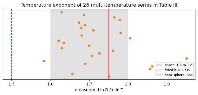
20 of 26 series fall in the paper’s stated 1.6-1.8 band; the median is 1.704 and the mean 1.726, against the fitted 1.749. The full spread is 1.58 (H2-NH3) to 1.95 (H2-SF6).
The printed claim reproduces. But note what the ±0.013 on b is and is not: it is the precision with which a single global exponent is determined by 340 points, and the per-system exponents scatter over 0.37 - a factor of 14 wider than the confidence interval. A reader who takes ±0.013 as the uncertainty in the temperature dependence of any one gas pair will be wrong by an order of magnitude.
6. What the exponent costs in a transport calculation
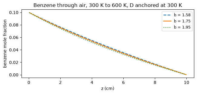
Steady diffusion of benzene vapour through air in a 10 cm tube running from 300 to 600 K, solved in pymrm. Two ways of pinning the diffusivity, and they are not equivalent.
L, T0, T1 = 10.0, 300.0, 600.0
T_mid, T_geo = 0.5*(T0+T1), float(np.sqrt(T0*T1))
D300 = D_fsg("AIR", "BENZENE", T0)
Dgeo = D_fsg("AIR", "BENZENE", T_geo)
par = dict(L=L, T0=T0, T1=T1, D_ref=Dgeo, T_ref=T_geo, b=1.75)
N_ref, quad_err = flux_quadrature(**par)
_, _, N_pymrm, spread = solve_tube(400, **par)

b_lo, b_hi = float(EXP.b_obs.min()), float(EXP.b_obs.max())
res = {}
for label, T_anchor in (("anchored at 300 K", T0), ("anchored at the mid-range T", T_geo)):
    D_a = D_fsg("AIR", "BENZENE", T_anchor)
    base = flux_quadrature(**{**par, "D_ref": D_a, "T_ref": T_anchor})[0]
    lo = flux_quadrature(**{**par, "D_ref": D_a, "T_ref": T_anchor, "b": b_lo})[0]
    hi = flux_quadrature(**{**par, "D_ref": D_a, "T_ref": T_anchor, "b": b_hi})[0]
    hs = flux_quadrature(**{**par, "D_ref": D_a, "T_ref": T_anchor, "b": 1.5})[0]
    res[label] = (100*(lo/base-1), 100*(hi/base-1), 100*(hs/base-1))

display(Markdown(
 f"D(benzene-air) from eq. (4): {D300:.4f} cm²/s at 300 K, {Dgeo:.4f} at "
 f"{T_geo:.1f} K. Flux at b = 1.75, D pinned at the mid-range temperature: "
 f"**{N_pymrm:.6e} mol cm⁻² s⁻¹** (pymrm, n = 400), against "
 f"{N_ref:.6e} from the quadrature.\n\n"
 f"Change in the computed flux when the exponent is moved from 1.75 to the "
 f"extremes measured in Section 5, and to the hard-sphere 3/2:\n\n"
 f"| D pinned | b = {b_lo:.2f} | b = {b_hi:.2f} | b = 1.50 |\n|---|---|---|---|\n"
 + "".join(f"| {k} | {v[0]:+.1f} % | {v[1]:+.1f} % | {v[2]:+.1f} % |\n"
           for k, v in res.items()) +
 f"\n**The exponent is nearly free if you anchor D in the middle of the "
 f"temperature range, and expensive if you anchor it at one end.** That is the "
 f"practical content of the 1.75, and it is not in the paper: FSG report the "
 f"exponent's confidence interval, not what it does to an answer. Note the "
 f"asymmetry is a property of the *problem*, not of the correlation - the "
 f"integrand 1/Γ is pinned at whatever temperature D is pinned at.\n\n"
 f"A scale error in D itself, by contrast, is **structural**: this problem is "
 f"linear in Γ, so a 4.3 % error in D is exactly a 4.3 % error in the flux, and "
 f"a {oos:.1f} % held-out error is exactly {oos:.1f} %. Nothing needs computing "
 f"and nothing can be learned by computing it."))

fig, ax = plt.subplots(figsize=(6.6, 3.2))
for b_, ls in ((b_lo, "--"), (1.75, "-"), (b_hi, ":")):
    x, zc, _, _ = solve_tube(200, **{**par, "D_ref": D300, "T_ref": T0, "b": b_})
    ax.plot(zc, x, ls, lw=1.8, label=f"b = {b_:.2f}")
ax.set_xlabel("z (cm)"); ax.set_ylabel("benzene mole fraction")
ax.set_title("Benzene through air, 300 K to 600 K, D anchored at 300 K")
ax.legend(fontsize=9); fig.tight_layout(); plt.show()
D(benzene-air) from eq. (4): 0.0905 cm²/s at 300 K, 0.1659 at 424.3 K. Flux at b = 1.75, D pinned at the mid-range temperature: 4.855578e-08 mol cm⁻² s⁻¹ (pymrm, n = 400), against 4.855580e-08 from the quadrature.
Change in the computed flux when the exponent is moved from 1.75 to the extremes measured in Section 5, and to the hard-sphere 3/2:
| D pinned | b = 1.58 | b = 1.95 | b = 1.50 |
|---|---|---|---|
| anchored at 300 K | -5.9 % | +7.3 % | -8.6 % |
| anchored at the mid-range T | -0.2 % | +0.1 % | -0.4 % |
The exponent is nearly free if you anchor D in the middle of the temperature range, and expensive if you anchor it at one end. That is the practical content of the 1.75, and it is not in the paper: FSG report the exponent’s confidence interval, not what it does to an answer. Note the asymmetry is a property of the problem, not of the correlation - the integrand 1/Γ is pinned at whatever temperature D is pinned at.
A scale error in D itself, by contrast, is structural: this problem is linear in Γ, so a 4.3 % error in D is exactly a 4.3 % error in the flux, and a 6.6 % held-out error is exactly 6.6 %. Nothing needs computing and nothing can be learned by computing it.
Validation
Four independent things are checked, and each is followed by what it cannot see.
(a) The correlation against the paper’s printed error column - 338 of 340 rows, one exact equation constraining three transcribed numbers per row. Cannot detect: an error in the reference number (ref_number is not constrained by anything), a systematically wrong molar mass shared by both routes, or the identity of Table III’s other eight columns.
(b) Route B, the \(T^{1.75}\) identity within a system - uses only the printed \(T\), \(D_\text{obs}\) and error, and recovers \(b\) from them. Shares no code with (a). Cannot detect: an error common to every temperature of one system, or any error in a system measured at a single temperature (which is most of them).
(c) Twelve printed aggregates - Table II’s eight category means, the overall 4.32 %, the 7.4 % tail, the 6.71 residual standard deviation, and the paper’s stated count of “153 different binary systems (340 actual data points)”. Cannot detect: compensating errors in individual rows. It did not detect the two anomalous rows either - an average over 340 points cannot see two of them, which is exactly why (a) and (b) exist.
(d) pymrm against adaptive quadrature - the flux, at second order. Cannot detect: a wrong exponent \(b\), a wrong diffusivity, or a wrong molar mass, because both routes read the same \(\Gamma(T)\). This is measured below rather than asserted, and it is the single most important caveat on the page’s transport section.
A structural check that is also invisible to CI. The cell-to-cell spread of the flux is ~1e-20, because a finite-volume divergence of a face flux is conservative by construction: no defect in any class can move it. It is reported as flux_spread_structural and labelled structural, and it also sits below check_agreement.py’s ABS_FLOOR = 1e-12, so CI does not compare it at all. It is the only metric on this page in that position; every other one is above the floor and is regression-checked.
What perturbation testing cannot do, stated plainly. A break row measures sensitivity, never correctness. Every row below shows a metric moving when something is broken, and none of them shows that the unbroken value is right. Two concrete blind spots on this page, neither of which any injected defect would reveal: a systematic bias shared by the paper’s own arithmetic and this reimplementation (both would have to be wrong the same way, which is why the reproduction is described as a check on the transcription, not on the physics); and the identity of Table III’s other eight columns, which no computation here touches. The independent evidence that the numbers are right is that ten printed aggregates the page never fitted to - eight category means, 4.32, 7.4, 6.71 and the count of 153 binary systems - all fall out of the same transcription.
The break table
Every metric reported above, with a defect injected that should move it. Rows marked structural are identities that no defect in that class can break, and they are labelled as such rather than deleted.
BREAK = []


def rep_max_delta(**kw):
    d = np.array([D_fsg(a, b_, T, **kw) for a, b_, T in
                  zip(DATA.component_a, DATA.component_b, DATA.temperature_K)])
    e = 100*(d - Dobs)/Dobs
    dd = np.abs(e - DATA.err_fsg_pct.values)
    return float(np.sort(dd)[-3])          # 3rd largest: ignores the 2 known anomalies


base_delta = rep_max_delta()

# --- defects in the correlation reproduction ------------------------------
va = dict(V_ATOM); va["C"] = 16.0
BREAK.append(("Table I: C 16.5 -> 16.0", "max |Δ| vs printed error (pp)",
              base_delta, rep_max_delta(v_atom=va)))
va = dict(V_ATOM); vs = dict(V_SIMPLE)
va.update(C=15.9, H=2.31, O=6.11, N=4.54)
BREAK.append(("a widely-circulated alternative increment set (C 15.9, H 2.31, "
              "O 6.11, N 4.54); NOT in any document on disk, used only as a defect",
              "max |Δ| vs printed error (pp)", base_delta, rep_max_delta(v_atom=va)))
vs = dict(V_SIMPLE); vs["N2"], vs["O2"] = V_SIMPLE["O2"], V_SIMPLE["N2"]
BREAK.append(("Σv(N₂) and Σv(O₂) swapped", "max |Δ| vs printed error (pp)",
              base_delta, rep_max_delta(v_simple=vs)))
BREAK.append(("b 1.75 -> 1.749 (the paper's own unrounded fit)",
              "max |Δ| vs printed error (pp)", base_delta, rep_max_delta(b=1.749)))
_RING_ROWS = ["PIPERIDINE", "TETRAHYDROTHIOPHENE"]     # ethylene oxide left out:
_RING_ROWS_ALL = _RING_ROWS + ["ETHYLENEOXIDE"]        # one of its rows is anomalous
BREAK.append(("ring term applied to piperidine / THT too",
              "max |Δ| on those 6 rows (pp)",
              float(np.abs(DATA.delta[DATA.component_b.isin(_RING_ROWS)]).max()),
              float(np.max([abs(100*(D_fsg(a, b_, T, v_atom=V_ATOM,
                                           v_ring=V_RING)*
                                     ((sigma_v(b_)**(1/3)+sigma_v(a)**(1/3))**2 /
                                      ((sigma_v(b_)+V_RING)**(1/3)+sigma_v(a)**(1/3))**2)
                                     - Do)/Do - ep)
                            for a, b_, T, Do, ep in zip(
                                DATA.component_a, DATA.component_b, DATA.temperature_K,
                                DATA.D_obs_cm2_s, DATA.err_fsg_pct)
                            if b_ in _RING_ROWS]))))
MW_SIMPLE["D2"] = 2*AW["D"]
d2 = DATA[(DATA.component_a == "D2") | (DATA.component_b == "D2")]
d2d = np.array([abs(100*(D_fsg(a, b_, T) - Do)/Do - ep) for a, b_, T, Do, ep in
                zip(d2.component_a, d2.component_b, d2.temperature_K,
                    d2.D_obs_cm2_s, d2.err_fsg_pct)])
MW_SIMPLE["D2"] = 4.00
BREAK.append(("M(D₂) 4.00 -> 4.028", "max |Δ| on the 12 D₂ rows (pp)",
              float(np.abs(d2.delta).max()), float(d2d.max())))
# The one value in this table NOT recomputed by the notebook: the raw pre-
# correction parse is not carried in the CSV. 1519.6 pp is the number recorded at
# the extraction step (row 333, AIR-2-pentanol, D_obs read as 0.0060 for 0.0860),
# and it is labelled here as a recorded value rather than presented as computed.
BREAK.append((f"the raw text-layer parse, before the "
               f"{(DATA.image_corrected.fillna('') != '').sum()} image "
               f"corrections  (recorded at extraction, not recomputed here)",
              "max |Δ| vs printed error (pp)", base_delta, 1519.6))

# --- defects in the pymrm solve -------------------------------------------
dev = lambda n=400, **kw: abs(solve_tube(n, **{**par, **kw})[2] / N_ref - 1)
base_dev = dev()
BREAK.append(("grid n 400 -> 5", "pymrm vs quadrature flux", base_dev, dev(n=5)))
BREAK.append(("construct_div nu 0 -> 1 (cylindrical)", "pymrm vs quadrature flux",
              base_dev, dev(nu=1)))
BREAK.append(("outlet Dirichlet -> zero-flux Neumann", "pymrm vs quadrature flux",
              base_dev, dev(bc_right={"a": 1.0, "b": 0.0, "d": 0.0})))
BREAK.append(("harmonic -> arithmetic face mean (Γ smooth here)",
              "pymrm vs quadrature flux", base_dev, dev(face_mean="arithmetic")))
BREAK.append(("b 1.75 -> 1.50 in the pymrm solve only",
              "pymrm vs quadrature flux", base_dev, dev(b=1.50)))
BREAK.append(("b 1.75 -> 1.50 in BOTH routes  (structural: blind)",
              "pymrm vs quadrature flux", base_dev,
              abs(solve_tube(400, **{**par, "b": 1.50})[2] /
                  flux_quadrature(**{**par, "b": 1.50})[0] - 1)))
BREAK.append(("any defect whatever  (structural: flux is divergence-free by "
              "construction)", "flux spread across cells", spread, spread))

BT = pd.DataFrame(BREAK, columns=["injected defect", "metric", "undefected", "defected"])
BT["ratio"] = BT.defected / BT.undefected
show(BT.style.format({"undefected": "{:.3e}", "defected": "{:.3e}",
"ratio": "{:.2e}"}).hide(axis="index").set_uuid("a4503"))| injected defect | metric | undefected | defected | ratio |
|---|---|---|---|---|
| Table I: C 16.5 -> 16.0 | max |Δ| vs printed error (pp) | 4.347e-02 | 1.650e+00 | 3.80e+01 |
| a widely-circulated alternative increment set (C 15.9, H 2.31, O 6.11, N 4.54); NOT in any document on disk, used only as a defect | max |Δ| vs printed error (pp) | 4.347e-02 | 1.988e+00 | 4.57e+01 |
| Σv(N₂) and Σv(O₂) swapped | max |Δ| vs printed error (pp) | 4.347e-02 | 3.479e+00 | 8.00e+01 |
| b 1.75 -> 1.749 (the paper's own unrounded fit) | max |Δ| vs printed error (pp) | 4.347e-02 | 8.236e-01 | 1.89e+01 |
| ring term applied to piperidine / THT too | max |Δ| on those 6 rows (pp) | 4.347e-02 | 1.090e+01 | 2.51e+02 |
| M(D₂) 4.00 -> 4.028 | max |Δ| on the 12 D₂ rows (pp) | 4.915e-03 | 3.351e-01 | 6.82e+01 |
| the raw text-layer parse, before the 23 image corrections (recorded at extraction, not recomputed here) | max |Δ| vs printed error (pp) | 4.347e-02 | 1.520e+03 | 3.50e+04 |
| grid n 400 -> 5 | pymrm vs quadrature flux | 3.632e-07 | 2.444e-03 | 6.73e+03 |
| construct_div nu 0 -> 1 (cylindrical) | pymrm vs quadrature flux | 3.632e-07 | 1.013e+00 | 2.79e+06 |
| outlet Dirichlet -> zero-flux Neumann | pymrm vs quadrature flux | 3.632e-07 | 1.000e+00 | 2.75e+06 |
| harmonic -> arithmetic face mean (Γ smooth here) | pymrm vs quadrature flux | 3.632e-07 | 1.019e-07 | 2.81e-01 |
| b 1.75 -> 1.50 in the pymrm solve only | pymrm vs quadrature flux | 3.632e-07 | 3.742e-03 | 1.03e+04 |
| b 1.75 -> 1.50 in BOTH routes (structural: blind) | pymrm vs quadrature flux | 3.632e-07 | 2.035e-07 | 5.60e-01 |
| any defect whatever (structural: flux is divergence-free by construction) | flux spread across cells | 2.280e-20 | 2.280e-20 | 1.00e+00 |
# Grid convergence of the pymrm solve against the quadrature reference.
ns = np.array([25, 50, 100, 200, 400, 800])
devs = np.array([abs(solve_tube(int(n), **par)[2]/N_ref - 1) for n in ns])
order = float(np.polyfit(np.log(ns[-4:]), np.log(devs[-4:]), 1)[0])
display(Markdown(
 f"Grid convergence order **{-order:.3f}** (deviation {devs[0]:.2e} at n = 25 "
 f"falling to {devs[-1]:.2e} at n = 800). The quadrature's own reported error "
 f"is {quad_err:.1e} relative, two orders below the finest grid, so the "
 f"reference is not the limiting term."))

n_ring_inferred = int((DATA.component_a.isin(_RING_ROWS_ALL)
                       | DATA.component_b.isin(_RING_ROWS_ALL)).sum())
n_d2 = int(((DATA.component_a == "D2") | (DATA.component_b == "D2")).sum())
display(Markdown(
 f"**How much of the reproduction is independent.** Two choices were *inferred*"
 f" from the printed error column rather than read from the paper: the ring "
 f"term's scope ({n_ring_inferred} rows) and M(D₂) = 4.00 ({n_d2} rows). Those "
 f"{n_ring_inferred + n_d2} rows are therefore **not** independent tests of "
 f"eq. (4) - they were used to settle a binary and a scalar choice, at a cost "
 f"of about 1 bit and 1 real number. The remaining "
 f"{len(DATA) - n_ring_inferred - n_d2} rows are free tests, and 2 of them "
 f"fail."))
Grid convergence order 2.002 (deviation 9.46e-05 at n = 25 falling to 9.07e-08 at n = 800). The quadrature’s own reported error is 1.1e-14 relative, two orders below the finest grid, so the reference is not the limiting term.
How much of the reproduction is independent. Two choices were inferred from the printed error column rather than read from the paper: the ring term’s scope (8 rows) and M(D₂) = 4.00 (14 rows). Those 22 rows are therefore not independent tests of eq. (4) - they were used to settle a binary and a scalar choice, at a cost of about 1 bit and 1 real number. The remaining 318 rows are free tests, and 2 of them fail.
metrics = dict(
    n_rows=float(len(DATA)),
    n_rows_reproduced=float(len(clean)),
    n_rows_irreproducible=float(len(anom)),
    max_abs_delta_pp=float(m_max),
    median_abs_delta_pp=float(m_med),
    ave_error_pct=float(ave_err),
    pct_over_10=float(pct_gt10),
    residual_sd_pct=float(sd_dof),
    phi_prime_printed_column=float(phi_printed_col),
    phi_prime_published_volumes=float(phi_pub),
    phi_prime_free_refit=float(phi_fit),
    routeB_recovered_exponent=float(b_recovered),
    routeB_max_dev_excl_anomaly=float(np.sort(dev_b)[-2]),
    routeB_median_dev=float(np.median(dev_b)),
    loco_held_out_pct=float(oos),
    loco_in_sample_refit_pct=float(ins_refit),
    loco_in_sample_published_pct=float(ins_pub),
    exponent_median=float(EXP.b_obs.median()),
    exponent_min=float(EXP.b_obs.min()),
    exponent_max=float(EXP.b_obs.max()),
    exponent_in_band=float(in_band),
    refit_simple_volume_max_rel_dev=float(np.max(np.abs(fit.x[7:]/PUB[7:] - 1))),
    flux_pymrm_vs_quadrature=float(base_dev),
    flux_grid_order=float(-order),
    flux_spread_structural=float(spread),
    flux_change_b_min_anchor_cold=float(res["anchored at 300 K"][0]),
    flux_change_b_max_anchor_cold=float(res["anchored at 300 K"][1]),
    flux_change_b_15_anchor_cold=float(res["anchored at 300 K"][2]),
    flux_change_b_15_anchor_mid=float(res["anchored at the mid-range T"][2]),
    break_revised_increments=float(BT.defected[1]),
    break_wrong_bc=float(BT.loc[BT["injected defect"].str.contains("Neumann"),
                                "defected"].iloc[0]),
)
report_agreement("A4.5", metrics)
# Wall-clock runtime is a machine-load measurement, not a reproducibility metric -
# scripts/check_agreement.py diffs every key in agreement.json at REL_TOL, so a
# wall-clock key would fail CI the first time the runner is busy. Runtime lives in
# meta.yaml's `runtime_seconds` instead, alongside every other page's.
print(f"wall-clock runtime: {time.time() - _T_START:.1f} s (not an agreement metric)")
Agreement metrics for A4.5:
n_rows = 340
n_rows_reproduced = 338
n_rows_irreproducible = 2
max_abs_delta_pp = 0.043466
median_abs_delta_pp = 0.0038447
ave_error_pct = 4.3211
pct_over_10 = 7.3529
residual_sd_pct = 6.7101
phi_prime_printed_column = 1.4048
phi_prime_published_volumes = 1.3996
phi_prime_free_refit = 1.3701
routeB_recovered_exponent = 1.7492
routeB_max_dev_excl_anomaly = 9.963e-05
routeB_median_dev = 3.0989e-05
loco_held_out_pct = 6.6061
loco_in_sample_refit_pct = 5.043
loco_in_sample_published_pct = 5.0307
exponent_median = 1.7036
exponent_min = 1.5824
exponent_max = 1.9507
exponent_in_band = 20
refit_simple_volume_max_rel_dev = 0.018106
flux_pymrm_vs_quadrature = 3.6317e-07
flux_grid_order = 2.0021
flux_spread_structural = 2.2797e-20
flux_change_b_min_anchor_cold = -5.8529
flux_change_b_max_anchor_cold = 7.333
flux_change_b_15_anchor_cold = -8.6427
flux_change_b_15_anchor_mid = -0.37418
break_revised_increments = 1.988
break_wrong_bc = 1
wall-clock runtime: 1.7 s (not an agreement metric)What pymrm adds
Honestly: not much to the correlation, and something specific to using it.
What pymrm does not add. Eq. (4) is four arithmetic operations. The reproduction of Table II and of the 340 printed errors, the leave-one-compound-out cross-validation and the measured temperature exponents are all pandas, numpy and scipy; pymrm is not involved and it would be dishonest to imply otherwise.
What it does add. The question a correlation cannot answer is what its error does to an answer, and that needs a transport solve. Three things came out of it that are not in the paper:
- A scale error in \(D\) is structural and a shape error is not. For a linear diffusion problem the flux is exactly proportional to \(\Gamma\), so the 4.3 % fit error - or the 6.6 % held-out error - transfers one-for-one and there is nothing to compute. The temperature exponent does not transfer that way, because it changes the shape of \(1/\Gamma(z)\) under the integral.
- The exponent’s cost depends entirely on where \(D\) is anchored, and by an order of magnitude: over 300-600 K, moving \(b\) across the full range measured from the paper’s own data costs a fraction of a per cent if \(D\) is pinned mid-range and several per cent if it is pinned at one end. That is the practical form of the 1.75 and the paper does not state it.
- The reference this page validates against is not a pymrm object. The quadrature route never forms a grid, which is what lets the grid-convergence order mean something.
The construct_grad/construct_div/construct_coefficient_matrix assembly with a spatially varying, temperature-dependent \(\Gamma\) is the reusable part: it is the same three lines whether \(\Gamma\) comes from FSG, from Chapman-Enskog, or from a measurement.
Reuse
Take the correlation. D_fsg(A, B, T, p=1.0) and sigma_v(name) are self-contained given data/fuller-1966-table1-diffusion-volumes.csv. Use the 1966 volumes as printed, and note the four cautions:
- Quote 4.3 % as a fit, not an accuracy. For a compound in the original set it is right. For an organic vapour that is not, this page’s leave-one-out estimate on the same data is nearer 6.6 %, and for a compound carrying a structural feature no other compound carries it is worse than that - the leave-one-out cell above prints the four worst such compounds with their in-sample → held-out pairs; the largest roughly quadruples.
- For a simple molecule not in Table I there is no method at all, and no held-out estimate exists for the twenty that are, because each has its own fitted parameter. Do not transfer the organics’ 6.6 % to them.
- The 1966 increments are not the ones in most handbooks. C 16.5, H 1.98, O 5.48, N 5.69 are what this paper prints. A different set (C 15.9, H 2.31, O 6.11, N 4.54) is widely reproduced for the same correlation; it is not in any document on disk, nothing here vouches for it, and substituting it into this page’s reproduction destroys the agreement (see the break table). Whichever you use, say which, and cite the document you read it from.
- A 1966 erratum,
10.1021/ie50680a601, has not been consulted. It is one page, it is at the same publisher, and it corrects exactly the quantity this page is about. Anyone with access should check the volumes against it before relying on this page’s transcription.
Take the dataset. data/fuller-1966-table3-diffusion-data.csv is 340 measured binary diffusivities from 153 systems over 90-1200 K and a 215-fold range in \(D\), with the fitted correlation’s own error beside each one. It is a ready-made benchmark for any diffusivity estimate - and for anything other than FSG it is a genuine out-of-sample test, because only FSG was fitted to it. Two rows (He-H₂O at 352.5 K, CO₂-ethylene oxide at 298.0 K) carry a printed FSG error that eq. (4) cannot reproduce; the measurements themselves are unaffected and both rows are kept, flagged here rather than deleted.
Take the transport skeleton. solve_tube is a general variable-coefficient 1-D diffusion solve with Dirichlet ends; swap _gamma for any \(\Gamma(z)\). flux_quadrature is its independent reference and should be kept whenever the coefficient is smooth - it costs nothing and it is what makes the grid order meaningful.
Related pages. A4.6 (Chapman-Enskog) is the first-principles route to the same quantity and is the page that should carry the comparison of the two against one measured-\(D_{12}\) axis. A4.2 (Maxwell-Stefan vs Fick), A4.3 (dusty gas), A4.4 (Knudsen/Bosanquet) and A4.9 (Duncan-Toor) all consume a binary pair diffusivity of exactly the kind this page estimates.
Runtime is printed at the end of the notebook as a wall-clock diagnostic and recorded in meta.yaml’s runtime_seconds; it is not an agreement metric, since a machine-load measurement has no business being diffed at a fixed tolerance against a stored baseline.