# Bootstrap: the pymrm this page was checked with, and the gallery files it was
# published with. Works in a checkout, in CI and on a fresh Colab VM.
GALLERY_REF = "gallery-2026.11.10.3"  # replaced by the release tag at publication
PYMRM = ">=3.4.0,<4"  # equals meta.yaml pymrm_min_version, up to the next major
PAGE = "A3.8-onda-correlations"  # equals the page directory

import os, sys, urllib.request
from pathlib import Path
_shared = next((p / "shared" for p in (Path.cwd(), *Path.cwd().parents)
                if (p / "shared" / "gallery_bootstrap.py").is_file()), None)
if _shared is None:
    _shared = (Path(os.environ.get("XDG_CACHE_HOME") or Path.home() / ".cache")
               / "pymrm-gallery" / GALLERY_REF)
    _shared.mkdir(parents=True, exist_ok=True)
    urllib.request.urlretrieve(
        "https://raw.githubusercontent.com/computational-chemical-engineering/"
        f"pymrm-gallery/{GALLERY_REF}/shared/gallery_bootstrap.py",
        _shared / "gallery_bootstrap.py")
sys.path.insert(0, str(_shared))
sys.modules.pop("gallery_bootstrap", None)
from gallery_bootstrap import setup
setup(PAGE, PYMRM, GALLERY_REF);  # the semicolon stops the cell echoing the path
The Onda correlations, and which of their fourteen constants the paper can see
sec:A
struct:S3
tier:T1
data:tier3
phase:gas-liquid
Three coupled correlations - wetted area, liquid-side and gas-side coefficients - with the area feeding the other two. The gas-side constants are pinned to 0.45 % by an identity the paper prints twice and never checks; the liquid-side exponent set turns out to cap the measured slope of k_L a against L at 0.800, and two of Onda’s own six runs sit above that cap. Every printed constant is then placed inside a pymrm counter-current absorber and its elasticity computed two ways, which is what shows that one exponent is inert wherever the packing and the liquid have the same surface tension.
The Onda correlations, and which of their fourteen constants the paper can see
Catalog ID: A3.8 · Structures: S3 (1D steady BVP) · Tier: T1
Onda, Takeuchi and Okumoto (1968) is the packed-column workhorse: three correlations that between them give the wetted area, the liquid-side coefficient and the gas-side coefficient, from packing geometry and fluid properties alone. It is still the default in process simulators.
Structurally it is not one correlation but three coupled ones, and the coupling runs one way: the wetted area \(a_w\) appears inside the liquid-side Reynolds number, so eq. (1) feeds eq. (2), while eq. (3) for the gas side is built on the total area and does not see \(a_w\) at all. That asymmetry is the whole reason the page is worth building, and it is where the interesting numbers turn out to be.
The page does four separate things and keeps them apart.
- Transcribes fourteen printed constants - eq. (3)’s prefactor is branched, so it is printed twice - and checks the transcription against a second printing of the same three equations inside the same PDF, the companion article that starts on journal page 62 restates all of them.
- Recovers eq. (4) from eq. (3). The authors rearrange the gas-side correlation into a \(j_D\) factor and print the result without showing the working. Redoing that working two independent ways gives 0.774443 against their printed 0.771, and the exponent to machine precision. It is the only check on this page that pins all four gas-side constants at once.
- Finds a ceiling the correlation cannot exceed. Combining eqs. (1) and (2) forces the local slope \(\mathrm{d}\ln(k_L a)/\mathrm{d}\ln L\) into the window \((2/3,\,0.8]\), for any packing, any liquid and any flow rate, because it depends on the exponent set alone and on no prefactor. Onda’s own Table 1 prints six measured slopes. Two of them, both spheres, are above the ceiling.
- Puts all fourteen constants inside a pymrm counter-current absorber and measures the elasticity of the packed height to each, analytically and by finite differences on the solved column. That is what shows which constants a design calculation can actually feel, and that one of them, \((\sigma_c/\sigma)^{0.75}\), is exactly inert whenever the packing’s critical surface tension equals the liquid’s.
What this page is not. Eqs. (2) and (3) were fitted to the very \(k_L a\) and \(k_G a\) data any comparison here would use, including Onda’s own Table 1 runs, which page 57 says were replotted against eq. (2) in Fig. 2. Nothing on this page is an out-of-sample test of those fits and nothing is labelled as one. The two comparisons that are free of that circularity are named where they occur: the eq. (4) identity, which is arithmetic the paper owes and never shows; and the exponent window, which no prefactor can move.
Background
Which paper this is, and how that was established. The file on disk is Onda1968-gas-liquid-mass-transfer-packed-columns-JCEJ1-56.pdf. A filename carries no verified metadata, so the article was identified by reading it. Journal page 56 carries the title “MASS TRANSFER COEFFICIENTS BETWEEN GAS AND LIQUID PHASES IN PACKED COLUMNS”, the byline “KAKUSABURO ONDA, HIROSHI TAKEUCHI** AND YOSHIO OKUMOTO / Dept. of Chem. Eng., University of Nagoya, Nagoya”, and the footnote “Received on July 10, 1967”. The running feet read “JOURNAL OF CHEMICAL ENGINEERING OF JAPAN” and “VOL.1 NO.1 1968”, and the printed folios run 56 to 62, so the filename encodes volume 1, page 56.
That reading was then checked against CrossRef for 10.1252/jcej.1.56, which returns the same title, the same three author surnames, container Journal of Chemical Engineering of Japan, volume 1, issue 1, pages 56–62, 1968. Title, authors, volume, issue, page range and year all agree with the page images, so the DOI is verified rather than auto-resolved from a terse citation.
Two other articles sit inside the same seven-page PDF and neither is used: page 56 opens with the last column of a preceding bubble-column paper, and page 62 begins “Gas absorption with chemical reaction in packed columns” by Onda, Sada and Takeuchi. That companion article earns exactly one job here, it reprints all three correlations verbatim in its introduction, giving a second, independently typeset printing against which every constant was checked.
Where the resolution rule bites. pdfimages -list reports all seven pages as CCITT-G4 bilevel, 2456 × 3330 px at 300 ppi native. Rendering at 600 dpi would interpolate and add nothing. Every equation and every table cell here was read from a 300 dpi render, cropped to a single line and re-read at that resolution, necessary because the 1968 typesetting sets exponents at roughly a quarter of body size, and at page scale -0.05 and 0.05, or -2.0 and -2.6, are not separable.
The problem Onda is solving. A packed absorption column has three unknowns a designer cannot measure: how much of the packing surface is actually wet, how fast the liquid film renews, and how fast the gas boundary layer transports. Most correlations of the day reported the product \(k_L a\) or \(k_G a\), coefficient times area, because that is what an experiment gives. Onda’s move, which he had been developing since 1959, was to correlate the area separately, then divide every published \(k_L a\) and \(k_G a\) by it to expose the bare coefficients. The first sentence of the paper says exactly that: “Assuming that the wetted surface on packing pieces is identical with the gas-liquid interface, Onda et al. presented the empirical equations of the gas and liquid-side mass transfer coefficients.”
That assumption is the load-bearing one. \(a_w\) is a wetted area, measured by wetting experiments; \(a\) is the interfacial area for mass transfer. Setting them equal is a modelling choice, and the paper’s own conclusion states it as one: “Assuming that the wetted surface area evaluated by Eq. (1) is identical with the gas-liquid interfacial area…”. Nothing on this page tests it, nothing in the paper can, because \(a_w\) never appears except multiplied by a coefficient.
Neighbouring pages. A3.1 (Whitman) is the two-film theory whose \(k_G\) and \(k_L\) these correlations supply; F3.1 (Hatta) and F3.5 cover what happens when reaction enhances the liquid film. A3.6 (Calderbank & Moo-Young) and A3.7 (van ’t Riet) are the stirred-tank analogues and are being built separately, neither is compared here. A3.9 (Billet–Schultes) and A3.10 (Rocha–Bravo–Fair) are the two later packed-column correlations that would make the natural three-way comparison with Onda; that comparison belongs to whichever of those two is built second, not here, because it needs their sources on disk and this page has only Onda’s.
The published model
Three correlations, in the paper’s own numbering and its own unit system (m, kg, hr, kg-mole, atm, K).
Eq. (1), wetted area (page 56, carried over from ref. 18, Onda, Takeuchi & Koyama 1967):
\[\frac{a_w}{a_t} \;=\; 1-\exp\left\{-1.45\left(\frac{\sigma_c}{\sigma}\right)^{0.75} \left(\frac{L}{a_t\mu_L}\right)^{0.1} \left(\frac{L^2 a_t}{\rho_L^2 g}\right)^{-0.05} \left(\frac{L^2}{\rho_L\sigma a_t}\right)^{0.2}\right\} \tag{1}\]
which the paper immediately re-writes as \(1-\exp\{-1.45(\sigma_c/\sigma)^{0.75}(Re)^{0.1}(Fr)^{-0.05}(We)^{0.2}\}\), naming the three groups. \(\sigma_c\) is the critical surface tension of the packing material, \(\sigma\) that of the liquid.
Eq. (2), liquid-side coefficient (page 57):
\[k_L\left(\frac{\rho_L}{\mu_L g}\right)^{1/3} = 0.0051\left(\frac{L}{a_w\mu_L}\right)^{2/3} \left(\frac{\mu_L}{\rho_L D_L}\right)^{-1/2} \left(a_t D_p\right)^{0.4} \tag{2}\]
Note the \(a_w\) in the Reynolds number. That is the coupling: eq. (1) feeds eq. (2), and it is why \(k_L\) is not a power law in \(L\).
Eq. (3), gas-side coefficient (page 58):
\[\frac{k_G R T}{a_t D_G} = 5.23\left(\frac{G}{a_t\mu_G}\right)^{0.7} \left(\frac{\mu_G}{\rho_G D_G}\right)^{1/3} \left(a_t D_p\right)^{-2.0} \tag{3}\]
Eq. (3) is branched. Page 58: “In Fig. 3, data for Raschig rings and Berl saddles smaller than 15 mm are situated on the lower group and are best correlated by merely changing the constant, 5.23, in Eq. (3) into 2.00.” The Conclusion on page 61 restates the criterion as “Raschig rings smaller than 15 mm and Berl saddles smaller than 1/2”“, and page 60 adds that for 1/2-in spheres under vaporization ”the constant of Eq.(3) might be changed into 2.00”. The paper gives no mechanism, “this cause is not clear at present”, only the observation that \(k_G a\) for packings below 15 mm falls with increasing \(a_t\). Both branches are exercised below.
Eq. (4), the same thing as a \(j_D\) factor (page 58). The authors note that \(a_t D_p = 6(1-\varepsilon) = 3.4\) for spheres and state, without showing the rearrangement,
\[j_D = 0.771\left[\frac{G D_p'}{\mu_G(1-\varepsilon)}\right]^{-0.30} \tag{4}\]
with \(D_p'\) “diameter of sphere possessing the same surface area as a piece of packing”. Eq. (4) is eq. (3) in different clothes, so it is an identity the paper owes and never displays, and recovering it is the strongest check available here.
Eq. (5), somebody else’s data (page 59). Shulman et al. (1955) correlated the sublimation of dry naphthalene packings, a gas-solid experiment with no liquid in it at all, as
\[j_D = 1.195\left[\frac{G D_p'}{\mu_G(1-\varepsilon)}\right]^{-0.36} \tag{5}\]
and Onda remarks that “the agreement between Eqs. (4) and (5) is fairly good within the region of \(100 < GD_p'/\mu_G(1-\varepsilon) < 10{,}000\)”. That sentence is the one comparison in the paper against data the authors did not fit, and it is quantified below.
Eq. (6), the design equation (page 60):
\[Z = G_M\int_{y_1}^{y_2}\left(\frac{1}{k_G a} +\frac{m}{k_L a\,c_{av}}\right)\frac{\mathrm{d}y}{y^{*}-y} \tag{6}\]
with \(G_M\) assumed constant and \(m\) the slope of the equilibrium line. This is resistance-in-series (A3.1) integrated down a column, and it is what the pymrm section below solves as a two-point boundary-value problem instead of a quadrature.
Parameters and assumptions
Units. Onda’s Nomenclature (page 61, continued on 62) fixes the system, and it is not SI: \(a\) in m²/m³, \(D\) in m²/hr, \(g\) in m/hr², \(G\) and \(L\) in kg/(m² hr), \(\mu\) in kg/(m hr), \(\rho\) in kg/m³, \(R\) in m³ atm/(kg-mole K), \(k_G\) in kg-mole/(m² hr atm), \(k_L\) in m/hr. Everything below works in those units. The one trap: the Weber group \(L^2/(\rho_L\sigma a_t)\) is dimensionless only if \(\sigma\) is in kg/hr², and page 62’s Nomenclature says exactly that, “\(\sigma\) = surface tension [dynes/cm] or [kg/hr²]”. The ratio \(\sigma_c/\sigma\) is unaffected. The notebook checks all three groups for dimensionlessness symbolically rather than trusting this paragraph.
What the paper does not print, and what is done about it.
- \(a_t\) for any named packing. Not tabulated anywhere. But the paper does print the sphere relation \(a_t D_p = 6(1-\varepsilon) = 3.4\), so every calculation on this page that needs a geometry uses spheres, with \(a_t\) and \(\varepsilon\) taken from that printed statement and from nothing else.
- \(\sigma_c\) for any packing material. Not printed in this article; it lives in ref. 18. So \(\sigma_c/\sigma\) is carried as an explicit page parameter, set to 0.85 for the base case and swept from 0.5 to 1.5 below. That value is a page choice and is labelled as one everywhere it is used; the sweep says what it costs. It also produces the page’s cleanest negative result: at \(\sigma_c/\sigma = 1\) the exponent 0.75 becomes exactly inert.
- The \(L\) range of Table 1’s runs. Not printed; Fig. 2’s abscissa is \(Re_L\), not \(L\). So the Table 1 comparison uses only the structural window, which needs no \(L\), no \(a_t\) and no property at all.
The illustrative absorber is not Onda’s. The pymrm column below needs fluid properties, and Onda publishes none. Air and water at 25 °C are used, from standard property tables, at gas and liquid loadings inside the ranges the paper itself prints for its vaporization runs (\(L\) = 5000–8000 kg/(m² hr), Figs. 4 and 6). No metric derived from that column is a claim about the paper. The column exists to make all fourteen constants live simultaneously and to measure which of them a design calculation can feel; its elasticities are properties of the correlation set, and the two that matter, \(f_G\) and the wetting function \(\varphi\), are reported so the numbers can be re-scaled to any other case.
The modelling assumptions carried into the column.
- Dilute solute, so \(G_M\) and \(L_M\) are constant down the column (Onda’s own assumption in eq. (6): “the gas molar flow rate, \(G_M\), is assumed to be constant”).
- The total pressure is carried explicitly. Onda’s \(k_G\) is in kg-mole/(m² hr atm), so it multiplies a partial pressure; eq. (6)’s driving force is a mole fraction, \(\mathrm{d}y/(y^*-y)\). The two agree only at \(P = 1\) atm, which eq. (6) leaves implicit. This page writes the gas-side resistance as \(1/(P\,k_G a_w)\), which reduces to Onda’s at 1 atm and is the correct generalisation away from it. \(P\) = 1 atm everywhere below, so no number changes; the term is there so a reuser at 20 bar does not silently inherit a factor of twenty.
- A straight equilibrium line \(y^* = m x\). Onda’s Fig. 9 is precisely a study of what happens when \(m\) varies down a column; that is not attempted here and the page says so.
- \(a = a_w\), Onda’s assumption, untested here and untestable from this paper.
- Isothermal, no reaction, plug flow in both phases, no axial dispersion. Axial dispersion in a packed absorber is
A2.6’s subject, not this page’s.
The data
Three CSVs, all transcriptions of printed characters off 300 ppi renders, the scan’s native resolution, with every numeric cropped and re-read at that resolution. Nothing on this page is digitised; no pixel of any figure is measured, and the page needs none, because the paper prints its own constants, its own reduced table and its own error bands as numerals.
onda-1968-correlation-constants.csv, all fourteen constants and exponents of eqs. (1)–(3), plus the four of eqs. (4) and (5). Every constant used anywhere in this notebook is read from this file; none is typed into the code.onda-1968-table1.csv, the six rows of Table 1 (page 57), the authors’ own CO₂-into-organic-solvent runs reduced to \(k_L a = \alpha L^n\).onda-1968-stated-results.csv, the scalar claims printed in the text: the four error bands, \(a_t D_p = 6(1-\varepsilon) = 3.4\), the validity range of the eq. (4)/eq. (5) comparison, and the three liquid loadings printed in the captions and legends of Figs. 4 and 6.
Tier. The correlation constants are tier 6, the authors’ own fits. Table 1 reduces the authors’ own measurements, so it is tier 3 in origin, but it is not out-of-sample: page 57 states these runs were replotted against eq. (2) in Fig. 2. The page’s Table 1 comparison is therefore in-sample, and is presented as such. What makes it worth doing anyway is that the quantity compared, the exponent window, cannot be moved by any fit of any prefactor.
This page loads no other page’s dataset, so no cross-page reconciliation is owed. It is a deliberate choice: A3.1 holds Whitman’s HCl equilibrium data and A3.4 holds a digitised Sherwood-number scatter, and neither contains a packed- column mass velocity that could be compared with anything here.
import gallery_utils as gu
import numpy as np
import pandas as pd
import matplotlib.pyplot as plt
import sympy as sp
from scipy.integrate import quad
from pymrm import vanleer, stoic
from pymrm.checks import find_roots, observed_orders

plt.rcParams.update({"figure.dpi": 110, "axes.grid": True, "grid.alpha": 0.3})
np.set_printoptions(linewidth=120)

PAGE = "A3.8-onda-correlations"
K = gu.load_data("onda-1968-correlation-constants.csv", page=PAGE)
T1 = gu.load_data("onda-1968-table1.csv", page=PAGE)
SR = gu.load_data("onda-1968-stated-results.csv", page=PAGE).set_index("quantity")
print(gu.cite_data(gu.load_meta("onda-1968-correlation-constants.csv", page=PAGE)))
claims = gu.Claims(PAGE.split("-")[0])


def one_root(f, lo, hi, what, log=False, xtol=1e-14):
    '''The single root of f on the physical range [lo, hi]; raises unless exactly one.'''
    r = find_roots(f, lo, hi, log=log, xtol=xtol)
    if len(r["roots"]) != 1:
        raise ValueError(f"{what}: {r['message']} on [{lo:g}, {hi:g}]")
    return r["roots"][0]


def c(symbol):
    '''A constant Onda printed, by name. Nothing in this notebook types one.'''
    return float(K.loc[K.symbol == symbol, "value"].iloc[0])

def stated(q):
    '''A scalar Onda printed in his running text, by name.'''
    return float(SR.loc[q, "value"])

display(K)
display(T1)
Onda, K.; Takeuchi, H.; Okumoto, Y. (1968) — Journal of Chemical Engineering of Japan 1(1) 56-62 — doi:10.1252/jcej.1.56 — equations| equation | role | symbol | value | printed_as | page | term | |
|---|---|---|---|---|---|---|---|
| 0 | 1 | prefactor | C_aw | 1.450000 | 1.45 | 56 | exponential prefactor of the wetted-area equation |
| 1 | 1 | exponent | e_sigma | 0.750000 | 0.75 | 56 | (sigma_c/sigma) |
| 2 | 1 | exponent | e_Re_L | 0.100000 | 0.1 | 56 | Re_L = L/(a_t mu_L) |
| 3 | 1 | exponent | e_Fr_L | -0.050000 | -0.05 | 56 | Fr_L = L^2 a_t/(rho_L^2 g) |
| 4 | 1 | exponent | e_We_L | 0.200000 | 0.2 | 56 | We_L = L^2/(rho_L sigma a_t) |
| 5 | 2 | prefactor | C_kL | 0.005100 | 0.0051 | 57 | prefactor of the liquid-side coefficient |
| 6 | 2 | exponent | e_Re_Lw | 0.666667 | 2/3 | 57 | Re_Lw = L/(a_w mu_L) |
| 7 | 2 | exponent | e_Sc_L | -0.500000 | -1/2 | 57 | Sc_L = mu_L/(rho_L D_L) |
| 8 | 2 | exponent | e_atDp_L | 0.400000 | 0.4 | 57 | a_t D_p |
| 9 | 3 | prefactor | C_kG | 5.230000 | 5.23 | 58 | prefactor of the gas-side coefficient (upper g... |
| 10 | 3 | prefactor | C_kG_small | 2.000000 | 2.00 | 58 | prefactor for Raschig rings < 15 mm and Berl s... |
| 11 | 3 | exponent | e_Re_G | 0.700000 | 0.7 | 58 | Re_G = G/(a_t mu_G) |
| 12 | 3 | exponent | e_Sc_G | 0.333333 | 1/3 | 58 | Sc_G = mu_G/(rho_G D_G) |
| 13 | 3 | exponent | e_atDp_G | -2.000000 | -2.0 | 58 | a_t D_p |
| 14 | 4 | prefactor | C_jD_onda | 0.771000 | 0.771 | 58 | j_D prefactor obtained by rearranging Eq. (3) ... |
| 15 | 4 | exponent | e_jD_onda | -0.300000 | -0.30 | 58 | G D_p'/(mu_G (1-eps)) |
| 16 | 5 | prefactor | C_jD_shulman | 1.195000 | 1.195 | 59 | j_D prefactor of Shulman et al. for naphthalen... |
| 17 | 5 | exponent | e_jD_shulman | -0.360000 | -0.36 | 59 | G D_p'/(mu_G (1-eps)) |
| row | packing | size_printed | absorbent | temp_C | alpha | n | |
|---|---|---|---|---|---|---|---|
| 0 | 1 | Raschig ring | 10 mm | CCl4 | 25 | 0.1200 | 0.70 |
| 1 | 2 | Berl saddle | 1/2-in | CCl4 | 25 | 0.0862 | 0.73 |
| 2 | 3 | Sphere | 1/2-in | CCl4 | 25 | 0.0227 | 0.86 |
| 3 | 4 | Sphere | 1/2-in | CH3OH | 20 | 0.0735 | 0.76 |
| 4 | 5 | Sphere | 1-in | CH3OH | 20 | 0.0389 | 0.83 |
| 5 | 6 | Rod | 14 mm | CCl4 | 25 | 0.0930 | 0.70 |
The transcription, checked against a second printing
Eqs. (1)–(3) appear twice inside this PDF: once as eqs. (1), (2), (3) of the main article on pages 56–58, and again in the introduction of the companion article that begins on page 62, renumbered (there \(a_w\) is eq. 1, \(k_G\) eq. 2 and \(k_L\) eq. 3). The two printings were cropped and read independently, and agree character for character on all fourteen constants.
That is a genuine transcription check, two separate typesettings of the same equations, but it is worth being precise about what it cannot catch: a constant that was mis-set identically in both printings, which is one editorial event away. The eq. (4) identity below is the check that would catch that, because it tests the four gas-side constants against a fifth printed number derived from them.
# The fourteen constants of eqs. (1)-(3), as read from the two printings.
# Fourteen, not thirteen, because eq. (3) prints its prefactor twice: 5.23 and 2.00.
C_AW, E_SIG, E_RE_L, E_FR_L, E_WE_L = (c("C_aw"), c("e_sigma"), c("e_Re_L"),
                                       c("e_Fr_L"), c("e_We_L"))
C_KL, E_RE_LW, E_SC_L, E_ATDP_L = c("C_kL"), c("e_Re_Lw"), c("e_Sc_L"), c("e_atDp_L")
C_KG, C_KG_SMALL, E_RE_G, E_SC_G, E_ATDP_G = (c("C_kG"), c("C_kG_small"), c("e_Re_G"),
                                              c("e_Sc_G"), c("e_atDp_G"))
# eqs. (4) and (5), which are NEVER inputs - they are targets.
C_JD_ONDA, E_JD_ONDA = c("C_jD_onda"), c("e_jD_onda")
C_JD_SHUL, E_JD_SHUL = c("C_jD_shulman"), c("e_jD_shulman")

both = K[K.equation.isin([1, 2, 3])]
print(f"{len(both)} constants in eqs. (1)-(3), each read from two independent printings")
print("  eq. (1):", ", ".join(both[both.equation == 1].printed_as))
print("  eq. (2):", ", ".join(both[both.equation == 2].printed_as))
print("  eq. (3):", ", ".join(both[both.equation == 3].printed_as))
N_CONSTANTS = int(len(both))
14 constants in eqs. (1)-(3), each read from two independent printings
eq. (1): 1.45, 0.75, 0.1, -0.05, 0.2
eq. (2): 0.0051, 2/3, -1/2, 0.4
eq. (3): 5.23, 2.00, 0.7, 1/3, -2.0The three groups of eq. (1) are dimensionless, checked, not assumed
Onda’s unit system is unusual enough that this is worth verifying symbolically rather than by eye, and it is the check that catches a mis-read \(\rho_L^2\) or a dropped square. The Weber group is the interesting one: it closes only with \(\sigma\) in kg/hr², which is what page 62’s Nomenclature says.
M_, KG_, HR_, MOL_ = sp.symbols("m kg hr kgmole", positive=True)
U = dict(L=KG_/(M_**2*HR_), G=KG_/(M_**2*HR_), a_t=1/M_, mu=KG_/(M_*HR_),
         rho=KG_/M_**3, g=M_/HR_**2, sigma=KG_/HR_**2, D=M_**2/HR_)
groups = {
    "Re_L = L/(a_t mu_L)":            U["L"]/(U["a_t"]*U["mu"]),
    "Fr_L = L^2 a_t/(rho_L^2 g)":     U["L"]**2*U["a_t"]/(U["rho"]**2*U["g"]),
    "We_L = L^2/(rho_L sigma a_t)":   U["L"]**2/(U["rho"]*U["sigma"]*U["a_t"]),
    "Re_G = G/(a_t mu_G)":            U["G"]/(U["a_t"]*U["mu"]),
    "Sc = mu/(rho D)":                U["mu"]/(U["rho"]*U["D"]),
    "a_t D_p":                        U["a_t"]*M_,
    "k_L (rho_L/(mu_L g))^(1/3)":     (M_/HR_)*(U["rho"]/(U["mu"]*U["g"]))**sp.Rational(1, 3),
}
DIMLESS_ALL = True
for name, expr in groups.items():
    simp = sp.simplify(expr)
    ok = simp == 1
    DIMLESS_ALL &= bool(ok)
    print(f"   {name:<34} -> {simp}   {'dimensionless' if ok else 'NOT DIMENSIONLESS'}")
print(f"\nall seven groups dimensionless in Onda's unit system: {DIMLESS_ALL}")
print("The Weber group closes ONLY with sigma in kg/hr2, which is what page 62 states.")
Re_L = L/(a_t mu_L) -> 1 dimensionless
Fr_L = L^2 a_t/(rho_L^2 g) -> 1 dimensionless
We_L = L^2/(rho_L sigma a_t) -> 1 dimensionless
Re_G = G/(a_t mu_G) -> 1 dimensionless
Sc = mu/(rho D) -> 1 dimensionless
a_t D_p -> 1 dimensionless
k_L (rho_L/(mu_L g))^(1/3) -> 1 dimensionless
all seven groups dimensionless in Onda's unit system: True
The Weber group closes ONLY with sigma in kg/hr2, which is what page 62 states.PyMRM implementation
Two objects. First the correlation set itself, assembled once from the CSV constants; then Onda’s eq. (6) rebuilt as a counter-current two-point boundary value problem rather than a quadrature, which is what makes the packed height a solved quantity instead of an integral evaluated along an assumed operating line.
The correlations. OndaSet holds the three equations and the derived \(K_G a\). Every constant enters as a named argument with the CSV value as its default, so the break table further down can perturb any single one of the thirteen continuous parameters, the branch is a choice of value for C_kG, not a fourteenth argument, without touching the code that uses them.
The column. Gas flows up, liquid down, solute passes from gas to liquid. With \(z\) measured from the bottom and the fields \([\,y,\;x\,]\):
\[\frac{\mathrm{d}}{\mathrm{d}z}\bigl(G_M\,y\bigr) = -N, \qquad \frac{\mathrm{d}}{\mathrm{d}z}\bigl(-L_M\,x\bigr) = +N, \qquad N = K_G a\,(y - m x),\]
i.e. one divergence of a convective flux per phase with opposite velocities, plus a pointwise interphase source. That is exactly construct_convflux_upwind followed by construct_div, with a two-component velocity v = [[G_M, -L_M]], and it is why the two phases can live as two fields of one array rather than as two coupled solvers.
Boundary conditions, on the outward normal. bc is a 2-tuple of dicts \(a\,\partial\phi/\partial n + b\,\phi = d\) with \(n\) pointing out of the domain, and each entry is a per-field list because the two phases enter at opposite ends:
- at \(z=0\) (bottom): gas inlet, \(y = y_{in}\) →
a=0, b=1, d=y_in; liquid outlet, \(\mathrm{d}x/\mathrm{d}z = 0\) →a=1, b=0, d=0. - at \(z=Z\) (top): gas outlet, \(\mathrm{d}y/\mathrm{d}z = 0\) →
a=1, b=0, d=0; liquid inlet, \(x = x_{in}\) →a=0, b=1, d=x_in.
construct_div uses nu=0, the axial coordinate of a column of constant cross-section is Cartesian, not cylindrical; nu=1 would be the radial coordinate of the same column and is not what is being differentiated here.
Linear, then nonlinear. The source is linear in \((y, x)\), so with first-order upwind faces the whole discrete problem is one constant sparse matrix: the convection operator, plus a per-cell \(2\times2\) coupling block assembled once with construct_coefficient_matrix. That takes one sparse solve and no Newton iteration. Second order comes from van Leer limited faces, and the limiter makes the face values depend on the field, so that problem is nonlinear: ConvFluxTVD returns the limited fluxes with their exact Jacobian and newton (with monotone damping) solves it from the upwind solution, its success checked. Deferred correction (the limiter correction lagged on the factorised upwind matrix) is kept as a second route to the same discrete solution, and the column cell prints how the two compare. The outlet values are read at the faces with compute_boundary_values, and the Validation section measures their order on a grid ladder.
from model import HR, R_GAS, G_ACC, OndaSet, Absorber, column_closed_form, set_printed_constants

# The printed constants OndaSet defaults to, read from the CSV above.
set_printed_constants(C_aw=C_AW, e_sigma=E_SIG, e_Re_L=E_RE_L, e_Fr_L=E_FR_L, e_We_L=E_WE_L,
                      C_kL=C_KL, e_Re_Lw=E_RE_LW, e_Sc_L=E_SC_L, e_atDp_L=E_ATDP_L,
                      C_kG=C_KG, e_Re_G=E_RE_G, e_Sc_G=E_SC_G, e_atDp_G=E_ATDP_G)
The illustrative operating point
Air and water at 25 °C and 1 atm, on 1-in ceramic spheres, at liquid and gas loadings inside the ranges Onda prints for his own vaporization runs. The fluid properties are standard-table values and are not Onda’s; the geometry is his, because \(a_t D_p = 6(1-\varepsilon) = 3.4\) for spheres is printed on page 58 and is the only packing geometry this article supplies.
ATDP_SPHERES = stated("atDp_spheres")             # 3.4, printed on page 58
SIX = stated("sixteen_one_minus_eps")             # 6, from a_t D_p = 6(1-eps)
EPS_SPHERES = 1.0 - ATDP_SPHERES / SIX
D_P = 0.0254                                      # 1-in spheres: a size the paper packs with
A_T = ATDP_SPHERES / D_P

SIGMA_RATIO = 0.85    # sigma_c/sigma: a PAGE PARAMETER. Onda does not print sigma_c
                      # for any packing material in this article; it lives in ref. 18.

PROPS = dict(  # air / water at 25 C, 1 atm, from standard tables - NOT from Onda
    rho_L=997.0, mu_L=8.90e-4 * HR, D_L=1.92e-9 * HR, sigma=0.0720 * HR**2,
    rho_G=1.184, mu_G=1.84e-5 * HR, D_G=1.60e-5 * HR, T=298.15, P=1.0)

L_REF = stated("L_fig6_hi_kg_m2_hr")   # 8000 kg/(m2 hr), printed in Fig. 6's legend
G_REF = 2000.0                         # kg/(m2 hr), a page choice inside Fig. 6's abscissa
C_AV = PROPS["rho_L"] / 18.015         # kg-mole/m3 of water
G_M = G_REF / 28.96                    # kg-mole/(m2 hr), air
L_M = L_REF / 18.015                   # kg-mole/(m2 hr), water

onda = OndaSet(a_t=A_T, D_p=D_P, sigma_ratio=SIGMA_RATIO, **PROPS)
PSI_REF, AW_REF = onda.psi(L_REF), onda.a_w(L_REF)
KL_REF, KG_REF = onda.k_L(L_REF), onda.k_G(G_REF)

print(f"spheres, from the paper:  a_t D_p = {ATDP_SPHERES}  ->  eps = {EPS_SPHERES:.5f}, "
      f"a_t = {A_T:.2f} m2/m3 at D_p = {D_P*1000:.1f} mm")
print(f"Sc_L = {onda.Sc_L:.1f}   Sc_G = {onda.Sc_G:.4f}   sigma_c/sigma = {SIGMA_RATIO} (page parameter)")
print(f"\nat L = {L_REF:.0f}, G = {G_REF:.0f} kg/(m2 hr):")
print(f"   psi          = {PSI_REF:.5f}          (eq. 1's exponent argument)")
print(f"   a_w/a_t      = {AW_REF/A_T:.5f}          a_w = {AW_REF:.2f} m2/m3")
print(f"   k_L          = {KL_REF:.5f} m/hr    = {KL_REF/HR:.3e} m/s")
print(f"   k_G          = {KG_REF:.4f} kg-mole/(m2 hr atm)")
print(f"   G_M = {G_M:.3f}, L_M = {L_M:.3f} kg-mole/(m2 hr),  c_av = {C_AV:.3f} kg-mole/m3")
AW_FRACTION_REF = float(AW_REF / A_T)
spheres, from the paper: a_t D_p = 3.4 -> eps = 0.43333, a_t = 133.86 m2/m3 at D_p = 25.4 mm
Sc_L = 464.9 Sc_G = 0.9713 sigma_c/sigma = 0.85 (page parameter)
at L = 8000, G = 2000 kg/(m2 hr):
psi = 0.61111 (eq. 1's exponent argument)
a_w/a_t = 0.45725 a_w = 61.21 m2/m3
k_L = 0.33929 m/hr = 9.425e-05 m/s
k_G = 6.2680 kg-mole/(m2 hr atm)
G_M = 69.061, L_M = 444.074 kg-mole/(m2 hr), c_av = 55.343 kg-mole/m3Results
1. Eq. (4) is eq. (3) rearranged, and the rearrangement recovers 0.771
The paper writes eq. (4) with no working. The working is worth doing, because it is the only place where all four constants of eq. (3) are tested against a number printed independently of them.
One thing has to be assumed, and it is worth naming before the result. Onda’s Nomenclature defines \(j_D\) only as “mass transfer factor defined by Eq. (4)”, circularly, and it never prints the underlying definition. So the standard Chilton–Colburn form is assumed here, and the agreement below is what confirms the assumption rather than the other way round: any other convention would shift the prefactor by a fixed factor and could not land within half a percent. Using a molar velocity in place of the mass velocity, for instance, would move it by a molecular weight, a factor of about 29 for air, not 1.004.
Two further conventions, both from the paper’s own Nomenclature. \(D_p'\) in eqs. (4) and (5) is the “diameter of sphere possessing the same surface area as a piece of packing”, whereas eq. (3) uses \(D_p\), the “nominal size of packing”. For spheres the two coincide, which is the only geometry used anywhere on this page and the only one for which the paper supplies \(a_t D_p\), so nothing here depends on the distinction, but a reuser applying eq. (4) to Raschig rings must respect it.
Start from the standard Chilton–Colburn factor \(j_D = (k_c/u)\,Sc^{2/3}\). In Onda’s units the coefficient in m/hr is \(k_G R T\) and the superficial gas velocity is \(G/\rho_G\), so
\[j_D = \frac{k_G R T\,\rho_G}{G}\,Sc_G^{2/3}.\]
Substituting eq. (3) and using \(Sc_G = \mu_G/(\rho_G D_G)\), the product \(D_G\rho_G Sc_G\) collapses to \(\mu_G\), the leftover \(Sc\) powers cancel exactly, and the whole thing reduces to a pure Reynolds power:
\[j_D = 5.23\,Re_G^{-0.3}\,(a_t D_p)^{-2}. \]
Then \(a_t D_p = 6(1-\varepsilon)\) for spheres makes \(Re_G = X/6\) with \(X = G D_p/[\mu_G(1-\varepsilon)]\), so
\[j_D = 5.23\cdot 6^{0.3}\cdot 3.4^{-2}\; X^{-0.30}.\]
Two things are being tested at once. The exponent \(-0.30\) is \(0.7-1\) and tests only eq. (3)’s Reynolds exponent. The prefactor tests 5.23 and \(-2.0\) together. And the absence of any Schmidt number in eq. (4) is what tests the \(1/3\): had eq. (3)’s Schmidt exponent been anything else, \(j_D\) would still contain \(Sc\) and could not be a function of \(X\) alone.
Below, that is done twice. Route A is a symbolic reduction with sympy from eq. (3) as transcribed, with no hand substitution. Route B never does any algebra: it evaluates eq. (3) numerically at four thousand independent random combinations of \(G\), \(\mu_G\), \(\rho_G\), \(D_G\) and \(D_p\) spanning several decades each, forms \(j_D\) and \(X\), and regresses \(\ln j_D\) on \(\ln X\). If eq. (3)’s Schmidt exponent were not \(1/3\), Route B’s residual would not be zero, its sample spans Schmidt numbers from about 0.02 to 80.
_at, _DG, _G, _muG, _rhoG, _Dp, _eps = sp.symbols(
    "a_t D_G G mu_G rho_G D_p varepsilon", positive=True)
rng = np.random.default_rng(20260805)          # seeded: this page reports its value
NSAMP = 4000
gs = 10**rng.uniform(2.0, 4.0, NSAMP)
mus = 10**rng.uniform(-2.2, -1.2, NSAMP)
rhos = 10**rng.uniform(-0.7, 0.7, NSAMP)
dgs = 10**rng.uniform(-2.5, -1.0, NSAMP)
dps = 10**rng.uniform(-2.5, -1.3, NSAMP)


def jd_routes(C=C_KG, e_Re=E_RE_G, e_Sc=E_SC_G, e_atDp=E_ATDP_G, atDp=ATDP_SPHERES,
              cc_exp_B=2.0 / 3.0):
    """Eq. (4) from eq. (3) by both routes; every argument is a constant of the reduction.

    Route A reduces eq. (3) symbolically; Route B evaluates it at the random property
    combinations and regresses ln j_D on ln X. ``cc_exp_B`` is the Chilton-Colburn
    Schmidt exponent of Route B alone.
    """
    eps = 1.0 - atDp / SIX
    # ---- Route A: symbolic, from eq. (3) as transcribed -----------------------
    ReG, ScG = _G / (_at * _muG), _muG / (_rhoG * _DG)
    kG_RT = (sp.nsimplify(C) * ReG**sp.nsimplify(e_Re) * ScG**sp.nsimplify(e_Sc)
             * (_at * _Dp)**sp.nsimplify(e_atDp) * _at * _DG)              # eq. (3) -> k_G R T
    jD = sp.simplify(kG_RT * _rhoG / _G * ScG**sp.Rational(2, 3))           # Chilton-Colburn
    jD = sp.simplify(jD.subs(_at, SIX * (1 - _eps) / _Dp))                  # spheres
    X = _G * _Dp / (_muG * (1 - _eps))
    ratio = sp.powsimp(sp.expand_power_exp(sp.simplify(jD / X**sp.nsimplify(E_JD_ONDA))),
                       force=True)
    ratio = sp.simplify(ratio.subs(_eps, sp.nsimplify(eps)))
    free = sp.simplify(jD).free_symbols
    # the prefactor exists as a number only when j_D is a function of X alone
    pref_A = float(ratio) if not ratio.free_symbols else np.nan
    # ---- Route B: numeric, no algebra at all ---------------------------------
    ats = atDp / dps
    Scs = mus / (rhos * dgs)
    kk = C * (gs / (ats * mus))**e_Re * Scs**e_Sc * (ats * dps)**e_atDp * ats * dgs
    jDs = kk * rhos / gs * Scs**cc_exp_B
    Xs = gs * dps / (mus * (1.0 - eps))
    slope, lnA = np.polyfit(np.log(Xs), np.log(jDs), 1)
    resid = np.log(jDs) - (lnA + slope * np.log(Xs))
    return dict(
        jD_expr=sp.simplify(jD), ratio=ratio, free=free, Scs=Scs, Xs=Xs,
        sc_cancels=bool(({_rhoG, _DG} & free) == set()),
        jd_prefactor_symbolic=pref_A,
        jd_prefactor_numeric=float(np.exp(lnA)),
        jd_prefactor_dev_pct=100.0 * (pref_A / C_JD_ONDA - 1.0),
        jd_exponent_numeric=float(slope),
        jd_exponent_dev=abs(float(slope) - E_JD_ONDA),
        jd_two_routes_spread=abs(float(np.exp(lnA)) / pref_A - 1.0),
        jd_fit_max_resid=float(np.abs(resid).max()))


JD = jd_routes()
JD_PREFACTOR_SYMBOLIC = JD["jd_prefactor_symbolic"]
JD_PREFACTOR_NUMERIC, JD_EXPONENT_NUMERIC = JD["jd_prefactor_numeric"], JD["jd_exponent_numeric"]
JD_FIT_MAX_RESID, JD_ROUTE_SPREAD = JD["jd_fit_max_resid"], JD["jd_two_routes_spread"]
JD_PREFACTOR_DEV_PCT, JD_EXPONENT_DEV = JD["jd_prefactor_dev_pct"], JD["jd_exponent_dev"]
SC_CANCELS = JD["sc_cancels"]
print("Route A (sympy, no hand algebra)")
print(f"   j_D reduces to        {JD['jD_expr']}")
print(f"   j_D / X^({E_JD_ONDA})      = {sp.nsimplify(JD['ratio'])}  = {JD_PREFACTOR_SYMBOLIC:.6f}")
print(f"   free symbols left in j_D: {sorted(map(str, JD['free']))}")
print(f"   neither rho_G nor D_G survives, so Sc has cancelled exactly: {SC_CANCELS}")
print("   That cancellation is what tests eq. (3)'s 1/3: any other Schmidt exponent")
print("   would leave Sc in j_D, and eq. (4) could not be a function of X alone.")
print(f"\nRoute B ({NSAMP} random property combinations, seed 20260805)")
print(f"   Sc_G sampled over  {JD['Scs'].min():.4f} .. {JD['Scs'].max():.2f}     "
      f"X sampled over {JD['Xs'].min():.1f} .. {JD['Xs'].max():.0f}")
print(f"   prefactor  {JD_PREFACTOR_NUMERIC:.6f}     exponent  {JD_EXPONENT_NUMERIC:.10f}")
print(f"   worst residual of the single-variable fit: {JD_FIT_MAX_RESID:.3e}")
print(f"\n   two routes agree to {JD_ROUTE_SPREAD:.2e}")
print(f"   against Onda's printed eq. (4):")
print(f"      prefactor  {JD_PREFACTOR_SYMBOLIC:.6f}  vs printed {C_JD_ONDA}   "
      f"-> {JD_PREFACTOR_DEV_PCT:+.3f} %")
print(f"      exponent   {JD_EXPONENT_NUMERIC:.6f} vs printed {E_JD_ONDA}   "
      f"-> {JD_EXPONENT_DEV:.2e}")
Route A (sympy, no hand algebra)
j_D reduces to 0.248682121242021*mu_G**(3/10)/(D_p**(3/10)*G**(3/10)*(1 - varepsilon)**(17/10))
j_D / X^(-0.3) = 38722129605159/50000000000000 = 0.774443
free symbols left in j_D: ['D_p', 'G', 'mu_G', 'varepsilon']
neither rho_G nor D_G survives, so Sc has cancelled exactly: True
That cancellation is what tests eq. (3)'s 1/3: any other Schmidt exponent
would leave Sc in j_D, and eq. (4) could not be a function of X alone.
Route B (4000 random property combinations, seed 20260805)
Sc_G sampled over 0.0205 .. 82.51 X sampled over 10.8 .. 103312
prefactor 0.774443 exponent -0.3000000000
worst residual of the single-variable fit: 3.109e-15
two routes agree to 2.22e-16
against Onda's printed eq. (4):
prefactor 0.774443 vs printed 0.771 -> +0.447 %
exponent -0.300000 vs printed -0.3 -> 1.11e-16What that 0.45 % is. It is not experimental agreement and not a model test; it is the paper’s own arithmetic, redone. The gap is consistent with the authors having rounded at an intermediate step; the cell below prints what the two obvious intermediate roundings give, and then what the printed 0.771 would require of each constant taken alone. None of the four is implausible, so no claim is made that anything is mis-set, this is reported so a reader can see the size of the discrepancy against the size of each constant.
def jd_prefactor(C=C_KG, e_Re=E_RE_G, e_atDp=E_ATDP_G, atDp=ATDP_SPHERES, six=SIX):
    """Closed form of eq. (4)'s prefactor from eq. (3)'s constants."""
    return C * six**(1.0 - e_Re) * atDp**e_atDp

print("the two obvious intermediate roundings of the same product:")
print(f"   round (a_t D_p)^-2  to 3 s.f.: {C_KG * SIX**(1-E_RE_G):.6g} x "
      f"{round(ATDP_SPHERES**E_ATDP_G, 6):.4g} -> "
      f"{C_KG * SIX**(1-E_RE_G) * float(f'{ATDP_SPHERES**E_ATDP_G:.3g}'):.6f}")
print(f"   round C_kG*6^0.3    to 3 s.f.: {float(f'{C_KG * SIX**(1-E_RE_G):.3g}'):.4g} x "
      f"{ATDP_SPHERES**E_ATDP_G:.6g} -> "
      f"{float(f'{C_KG * SIX**(1-E_RE_G):.3g}') * ATDP_SPHERES**E_ATDP_G:.6f}")
print(f"   the paper prints {C_JD_ONDA}, which is below both.\n")

# Each inversion is the single root on the constant's physical range: the prefactor
# is monotone in each constant, so exactly one root is expected and anything else raises.
INVERT = [("C_kG   5.23", C_KG, "C", 0.5, 50.0),
          ("e_Re_G 0.7", E_RE_G, "e_Re", 0.0, 1.0),
          ("e_atDp_G -2.0", E_ATDP_G, "e_atDp", -4.0, 0.0),
          ("a_t D_p 3.4", ATDP_SPHERES, "atDp", 0.6, SIX)]   # eps from 0.9 down to 0
rows = [(lbl, v0, one_root(lambda v, k=k: jd_prefactor(**{k: v}) - C_JD_ONDA, lo, hi, lbl))
        for lbl, v0, k, lo, hi in INVERT]
alt = pd.DataFrame(rows, columns=["printed constant", "printed value",
                                  "value that would give exactly 0.771"])
alt["relative shift"] = alt["value that would give exactly 0.771"] / alt["printed value"] - 1
display(alt.round(6))
print("None of these is a plausible mis-reading of the page image, and the page")
print("claims no mis-set constant. What the row for a_t D_p shows is that the")
print("printed 3.4 is itself a rounding of 6(1-eps), which is the likeliest source.")
JD_ATDP_FOR_0771 = float(alt.loc[alt["printed constant"] == "a_t D_p 3.4",
                                 "value that would give exactly 0.771"].iloc[0])
print(f"\n   a_t D_p = {JD_ATDP_FOR_0771:.4f} reproduces 0.771 exactly; the paper prints 3.4,")
print(f"   i.e. eps = {1-JD_ATDP_FOR_0771/SIX:.5f} against the printed {EPS_SPHERES:.5f}.")
the two obvious intermediate roundings of the same product:
round (a_t D_p)^-2 to 3 s.f.: 8.95256 x 0.0865 -> 0.774396
round C_kG*6^0.3 to 3 s.f.: 8.95 x 0.0865052 -> 0.774221
the paper prints 0.771, which is below both.
| printed constant | printed value | value that would give exactly 0.771 | relative shift | |
|---|---|---|---|---|
| 0 | C_kG 5.23 | 5.23 | 5.206751 | -0.004445 |
| 1 | e_Re_G 0.7 | 0.70 | 0.702486 | 0.003552 |
| 2 | e_atDp_G -2.0 | -2.00 | -2.003641 | 0.001820 |
| 3 | a_t D_p 3.4 | 3.40 | 3.407582 | 0.002230 |
None of these is a plausible mis-reading of the page image, and the page
claims no mis-set constant. What the row for a_t D_p shows is that the
printed 3.4 is itself a rounding of 6(1-eps), which is the likeliest source.

   a_t D_p = 3.4076 reproduces 0.771 exactly; the paper prints 3.4,
   i.e. eps = 0.43207 against the printed 0.43333.
2. Eq. (4) against Shulman’s naphthalene, over the range the paper states
This is the one comparison in the article against data the authors did not fit. Eq. (5) comes from Shulman, Ullrich, Proulx and Zimmerman (1955), who sublimed dry naphthalene packings, a gas–solid experiment with no liquid, no wetted area and no absorption in it. Onda’s remark is that the two agree “fairly good” over \(100 < X < 10{,}000\), and gives no number.
The two are power laws with different exponents, so they can only cross once. The cell below puts the number on it, and reports the crossing.
XLO, XHI = stated("shulman_range_lo"), stated("shulman_range_hi")
Xg = np.logspace(np.log10(XLO), np.log10(XHI), 801)
j_onda = C_JD_ONDA * Xg**E_JD_ONDA
j_shul = C_JD_SHUL * Xg**E_JD_SHUL
ratio = j_onda / j_shul

# The ratio of two power laws is itself a power law, monotone in X, so its largest
# |deviation| over the range sits at a range end: the ends are evaluated at XLO and
# XHI themselves. The mean is over ln X (the plotted axis), integrated on either
# side of the crossing.
def eq45_ratio(X, c4=C_JD_ONDA, e4=E_JD_ONDA, c5=C_JD_SHUL, e5=E_JD_SHUL):
    return (c4 * X**e4) / (c5 * X**e5)

EQ45_DEV_LO_PCT = float(100.0 * (eq45_ratio(XLO) - 1.0))       # at the range end X = XLO
EQ45_DEV_HI_PCT = float(100.0 * (eq45_ratio(XHI) - 1.0))       # at the range end X = XHI
EQ45_MAX_DEV_PCT = max(abs(EQ45_DEV_LO_PCT), abs(EQ45_DEV_HI_PCT))
EQ45_CROSSOVER_X = float(np.exp(np.log(C_JD_SHUL / C_JD_ONDA) / (E_JD_ONDA - E_JD_SHUL)))
_dev = lambda lnX: abs(eq45_ratio(np.exp(lnX)) - 1.0)
EQ45_MEAN_DEV_PCT = float(100.0 * sum(
    quad(_dev, a, b, epsabs=0.0, epsrel=1e-12)[0]
    for a, b in ((np.log(XLO), np.log(EQ45_CROSSOVER_X)),
                 (np.log(EQ45_CROSSOVER_X), np.log(XHI)))) / np.log(XHI / XLO))
# null baseline: how much does j_D itself move over the same range (range ends)?
EQ45_ONDA_SPAN = float((XLO / XHI)**E_JD_ONDA)
EQ45_SHUL_SPAN = float((XLO / XHI)**E_JD_SHUL)

print(f"Eq. (4) / Eq. (5) over the paper's own stated range {XLO:.0f} < X < {XHI:.0f}:")
print(f"   at X = {XLO:8.0f}   {EQ45_DEV_LO_PCT:+7.2f} %   (Onda LOW)")
print(f"   at X = {EQ45_CROSSOVER_X:8.1f}      0.00 %   (they cross)")
print(f"   at X = {XHI:8.0f}   {EQ45_DEV_HI_PCT:+7.2f} %   (Onda HIGH)")
print(f"   worst |deviation| {EQ45_MAX_DEV_PCT:.2f} % (at a range end), "
      f"mean over ln X {EQ45_MEAN_DEV_PCT:.2f} %")
print(f"\nNULL BASELINE - what a constant j_D would achieve over the same range:")
print(f"   j_D itself falls by a factor {EQ45_ONDA_SPAN:.2f} (Onda) and "
      f"{EQ45_SHUL_SPAN:.2f} (Shulman) across those two decades,")
print(f"   so a single constant fitted to the mid-range is off by roughly a factor")
print(f"   {np.sqrt(EQ45_ONDA_SPAN):.2f} at each end - about {100*(np.sqrt(EQ45_ONDA_SPAN)-1):.0f} %,")
print(f"   against the {EQ45_MAX_DEV_PCT:.1f} % the two correlations differ by. That is what")
print(f'   "fairly good" is worth: better than a constant by a factor '
      f'{100*(np.sqrt(EQ45_ONDA_SPAN)-1)/EQ45_MAX_DEV_PCT:.1f}.')
print(f"\nThis is the only comparison on this page against data Onda did not fit -")
print("but note it is correlation against correlation, not correlation against")
print("measurement: Shulman's own scatter about eq. (5) is not printed here.")
Eq. (4) / Eq. (5) over the paper's own stated range 100 < X < 10000:
at X = 100 -14.95 % (Onda LOW)
at X = 1485.6 0.00 % (they cross)
at X = 10000 +12.12 % (Onda HIGH)
worst |deviation| 14.95 % (at a range end), mean over ln X 6.96 %
NULL BASELINE - what a constant j_D would achieve over the same range:
j_D itself falls by a factor 3.98 (Onda) and 5.25 (Shulman) across those two decades,
so a single constant fitted to the mid-range is off by roughly a factor
2.00 at each end - about 100 %,
against the 14.9 % the two correlations differ by. That is what
"fairly good" is worth: better than a constant by a factor 6.7.
This is the only comparison on this page against data Onda did not fit -
but note it is correlation against correlation, not correlation against
measurement: Shulman's own scatter about eq. (5) is not printed here.fig, ax = plt.subplots(1, 2, figsize=(10.4, 3.9))
ax[0].loglog(Xg, j_onda, "-", lw=1.8, color="C0",
label=f"Onda eq. (4): {C_JD_ONDA} X^{{{E_JD_ONDA}}}")
ax[0].loglog(Xg, j_shul, "--", lw=1.8, color="C3",
label=f"Shulman eq. (5): {C_JD_SHUL} X^{{{E_JD_SHUL}}}")
ax[0].axvline(EQ45_CROSSOVER_X, ls=":", color="0.5", lw=1)
ax[0].set_xlabel(r"$X = G D_p' / [\mu_G(1-\varepsilon)]$"); ax[0].set_ylabel(r"$j_D$")
ax[0].set_title("Two correlations, disjoint datasets"); ax[0].legend(fontsize=8)
ax[1].semilogx(Xg, 100 * (ratio - 1), "-", lw=1.8, color="C2")
ax[1].axhline(0, color="0.4", lw=1)
ax[1].axvline(EQ45_CROSSOVER_X, ls=":", color="0.5", lw=1)
ax[1].annotate(f"cross at X = {EQ45_CROSSOVER_X:.0f}", (EQ45_CROSSOVER_X, 0),
textcoords="offset points", xytext=(6, 16), fontsize=8)
ax[1].set_xlabel(r"$X$"); ax[1].set_ylabel("eq. (4) relative to eq. (5) / %")
ax[1].set_title(f'"fairly good" = {EQ45_MAX_DEV_PCT:.1f} % worst over the stated range')
fig.tight_layout(); plt.show()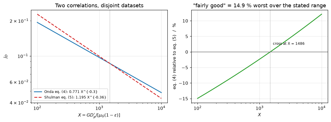
3. The exponent window, and where Onda’s own Table 1 sits
This is the page’s one comparison against measured numbers, and the one place the correlation can be caught out.
Onda’s Table 1 reduces each of the authors’ runs to a power law \(k_L a = \alpha L^{n}\). In his own framework \(a = a_w\), so the correlation predicts the same product:
\[k_L a_w \;\propto\; \left(\frac{L}{a_w}\right)^{2/3} a_w \;=\; L^{2/3}\,a_w^{1/3} \quad\Longrightarrow\quad n \;=\; \frac{2}{3} + \frac13\,\frac{\mathrm{d}\ln a_w}{\mathrm{d}\ln L}.\]
Now the \(L\)-dependence of eq. (1) collapses to a single composite exponent: \(Re\propto L\), \(Fr\propto L^2\), \(We\propto L^2\), so \(\psi \propto L^{\,0.1 + 2(-0.05) + 2(0.2)} = L^{0.4}\), and
\[\frac{\mathrm{d}\ln a_w}{\mathrm{d}\ln L} = 0.4\,\varphi(\psi),\qquad \varphi(\psi)=\frac{\psi e^{-\psi}}{1-e^{-\psi}} \in (0,1).\]
Therefore
\[\boxed{\;\frac23 \;<\; n \;\le\; \frac23+\frac{0.4}{3} = 0.8\;}\]
for every packing, every liquid and every flow rate. The bound involves no prefactor at all, not 1.45, not 0.0051, not \(\sigma_c/\sigma\), not \(a_t D_p\), not the Schmidt number. It is a property of the exponent set, so no fit can move it, which is exactly what makes it testable against a table those fits have already seen.
The window is derived twice below: from the algebra above, and by numerically differentiating the composed functions a_w(L) and k_L(L) as coded, with no reference to the derivation. A slip in either shows up as a disagreement.
# ---- Route A: the analytic window ----------------------------------------
L_COMPOSITE = E_RE_L + 2 * E_FR_L + 2 * E_WE_L      # 0.1 + 2(-0.05) + 2(0.2)
WINDOW_LO = E_RE_LW                                  # 2/3, as psi -> infinity
WINDOW_HI = E_RE_LW + L_COMPOSITE * (1.0 - E_RE_LW)  # 2/3 + 0.4/3, as psi -> 0
print(f"composite L-exponent of psi : {E_RE_L} + 2({E_FR_L}) + 2({E_WE_L}) = {L_COMPOSITE}")
print(f"window for n = dln(k_L a_w)/dlnL :  ({WINDOW_LO:.6f}, {WINDOW_HI:.6f})")

def n_pred_analytic(o, L):
    return E_RE_LW + L_COMPOSITE * (1.0 - E_RE_LW) * o.phi(L)

# ---- Route B: numerical differentiation of the coded functions -----------
def n_pred_numeric(o, L, rel=1e-5):
    lo, hi = L * (1 - rel), L * (1 + rel)
    f = lambda x: np.log(o.k_L(x) * o.a_w(x))
    return (f(hi) - f(lo)) / (np.log(hi) - np.log(lo))

Ls = np.logspace(np.log10(50.0), np.log10(500000.0), 240)
na = np.array([n_pred_analytic(onda, L) for L in Ls])
nb = np.array([n_pred_numeric(onda, L) for L in Ls])
N_WINDOW_TWO_ROUTES = float(np.abs(na - nb).max())
print(f"\nanalytic vs numerical-differentiation, over L = 50 .. 5e5 kg/(m2 hr): "
      f"worst {N_WINDOW_TWO_ROUTES:.3e}")
print(f"   numerically attained range of n over that sweep: "
      f"{nb.min():.6f} .. {nb.max():.6f}")
print(f"   psi over the same sweep: {onda.psi(Ls).min():.4g} .. {onda.psi(Ls).max():.4g}")
N_SWEEP_MIN, N_SWEEP_MAX = float(nb.min()), float(nb.max())
WINDOW_ESCAPE = float(max(0.0, nb.max() - WINDOW_HI, WINDOW_LO - nb.min()))
print(f"   the sweep never leaves the analytic window: escape = {WINDOW_ESCAPE:.2e}")
composite L-exponent of psi : 0.1 + 2(-0.05) + 2(0.2) = 0.4
window for n = dln(k_L a_w)/dlnL : (0.666667, 0.800000)
analytic vs numerical-differentiation, over L = 50 .. 5e5 kg/(m2 hr): worst 9.859e-11
numerically attained range of n over that sweep: 0.684864 .. 0.794721
psi over the same sweep: 0.08026 .. 3.195
the sweep never leaves the analytic window: escape = 0.00e+00n_meas = T1["n"].to_numpy(float)
inside = (n_meas > WINDOW_LO) & (n_meas <= WINDOW_HI)
tab = T1.copy()
tab["inside_window"] = inside
tab["excess_over_ceiling"] = np.maximum(0.0, n_meas - WINDOW_HI)
display(tab[["row", "packing", "size_printed", "absorbent", "n",
"inside_window", "excess_over_ceiling"]])
TABLE1_N_INSIDE = int(inside.sum())
TABLE1_N_TOTAL = int(len(n_meas))
TABLE1_WORST_EXCESS = float(np.maximum(0.0, n_meas - WINDOW_HI).max())
TABLE1_N_RANGE = float(n_meas.max() - n_meas.min())
print(f"\n{TABLE1_N_INSIDE} of {TABLE1_N_TOTAL} printed exponents lie inside "
f"({WINDOW_LO:.4f}, {WINDOW_HI:.4f})")
outs = tab[~inside]
for _, r in outs.iterrows():
print(f" OUTSIDE: row {int(r['row'])} {r['packing']} {r['size_printed']} "
f"in {r['absorbent']} n = {r['n']} -> {r['n']-WINDOW_HI:+.3f} above the ceiling")
print(f"\nworst excess over the ceiling: {TABLE1_WORST_EXCESS:+.3f}")
print(f"Table 1's n spans {TABLE1_N_RANGE:.2f}; the window is only "
f"{WINDOW_HI-WINDOW_LO:.4f} wide. The correlation's exponent set cannot")
print("generate the spread the authors' own six runs display.")| row | packing | size_printed | absorbent | n | inside_window | excess_over_ceiling | |
|---|---|---|---|---|---|---|---|
| 0 | 1 | Raschig ring | 10 mm | CCl4 | 0.70 | True | 0.00 |
| 1 | 2 | Berl saddle | 1/2-in | CCl4 | 0.73 | True | 0.00 |
| 2 | 3 | Sphere | 1/2-in | CCl4 | 0.86 | False | 0.06 |
| 3 | 4 | Sphere | 1/2-in | CH3OH | 0.76 | True | 0.00 |
| 4 | 5 | Sphere | 1-in | CH3OH | 0.83 | False | 0.03 |
| 5 | 6 | Rod | 14 mm | CCl4 | 0.70 | True | 0.00 |
4 of 6 printed exponents lie inside (0.6667, 0.8000)
   OUTSIDE: row 3  Sphere 1/2-in in CCl4   n = 0.86  -> +0.060 above the ceiling
   OUTSIDE: row 5  Sphere 1-in in CH3OH   n = 0.83  -> +0.030 above the ceiling

worst excess over the ceiling: +0.060
Table 1's n spans 0.16; the window is only 0.1333 wide. The correlation's exponent set cannot
generate the spread the authors' own six runs display.
Null baselines, beside it. A window is a prediction with no free parameters, so it must be scored against predictors that have none either, and against one that has a single fitted parameter, which is the honest hard case.
def mae(pred):
    return float(np.abs(n_meas - pred).mean())

BEST_CONST = float(np.median(n_meas))     # the 1-parameter null, MAE-optimal
MAE_WINDOW_TOP = mae(WINDOW_HI)           # Onda at his own ceiling, 0 free parameters
MAE_WINDOW_MID = mae(0.5 * (WINDOW_LO + WINDOW_HI))
MAE_NULL_23 = mae(WINDOW_LO)              # drop the wetted-area coupling entirely
MAE_NULL_1 = mae(1.0)                     # k_L a proportional to L
MAE_NULL_FITTED = mae(BEST_CONST)         # 1 fitted parameter on 6 points

scores = pd.DataFrame([
    ("Onda, at the window ceiling n = 0.800", 0, MAE_WINDOW_TOP),
    ("Onda, at the window midpoint", 0, MAE_WINDOW_MID),
    ("null: n = 2/3, i.e. NO wetted-area coupling", 0, MAE_NULL_23),
    ("null: n = 1, k_L a proportional to L", 0, MAE_NULL_1),
    (f"null: best constant, fitted = {BEST_CONST:.4f}", 1, MAE_NULL_FITTED),
], columns=["predictor", "free parameters", "mean |error| in n"])
display(scores.round(5))
print(f"Onda's ceiling has a mean |error| {MAE_NULL_23/MAE_WINDOW_TOP:.2f} times smaller than "
      "the no-coupling null.")
print(f"A single fitted constant, {BEST_CONST:.4f}, has one {MAE_WINDOW_TOP/MAE_NULL_FITTED:.2f} "
      "times smaller than Onda's ceiling.")

def paired_t(pred_a, pred_b):
    """Mean of |error of a| - |error of b| over the six rows, over its standard error."""
    d = np.abs(n_meas - pred_a) - np.abs(n_meas - pred_b)
    return float(d.mean() / (d.std(ddof=1) / np.sqrt(d.size)))

def one_sample_t(x):
    """Mean of x over its standard error."""
    return float(x.mean() / (x.std(ddof=1) / np.sqrt(x.size)))

T_N_ABOVE_NO_COUPLING = one_sample_t(n_meas - WINDOW_LO)     # exponents minus 2/3
T_CEILING_VS_NO_COUPLING = paired_t(WINDOW_LO, WINDOW_HI)   # > 0: the ceiling is better
T_FITTED_VS_CEILING = paired_t(WINDOW_HI, BEST_CONST)        # > 0: the fitted constant is better
print(f"\nEvery exponent above 2/3: one-sample t of (n - 2/3) = {T_N_ABOVE_NO_COUPLING:.2f} "
      f"on {n_meas.size - 1} degrees of freedom")
print("Each gap in mean |error| over its standard error (paired over the six rows):")
print(f"   ceiling against no coupling:        t = {T_CEILING_VS_NO_COUPLING:.2f}")
print(f"   fitted constant against the ceiling: t = {T_FITTED_VS_CEILING:.2f}")
print("With six rows, no replicates and no error bars on n, a t below 2 does not")
print("separate two predictors. It bounds what this table can establish, which is")
print("less than the window's cleanliness suggests.")| predictor | free parameters | mean |error| in n | |
|---|---|---|---|
| 0 | Onda, at the window ceiling n = 0.800 | 0 | 0.06667 |
| 1 | Onda, at the window midpoint | 0 | 0.05333 |
| 2 | null: n = 2/3, i.e. NO wetted-area coupling | 0 | 0.09667 |
| 3 | null: n = 1, k_L a proportional to L | 0 | 0.23667 |
| 4 | null: best constant, fitted = 0.7450 | 1 | 0.05333 |
Onda's ceiling has a mean |error| 1.45 times smaller than the no-coupling null.
A single fitted constant, 0.7450, has one 1.25 times smaller than Onda's ceiling.

Every exponent above 2/3: one-sample t of (n - 2/3) = 3.50 on 5 degrees of freedom
Each gap in mean |error| over its standard error (paired over the six rows):
   ceiling against no coupling:        t = 0.80
   fitted constant against the ceiling: t = 0.60
With six rows, no replicates and no error bars on n, a t below 2 does not
separate two predictors. It bounds what this table can establish, which is
less than the window's cleanliness suggests.
fig, ax = plt.subplots(figsize=(7.6, 4.2))
psis = np.logspace(-3, 2, 400)
phi = psis * np.exp(-psis) / (1 - np.exp(-psis))
ax.semilogx(psis, E_RE_LW + L_COMPOSITE * (1 - E_RE_LW) * phi, "-", lw=2, color="C0",
label=r"Onda: $n = 2/3 + 0.4\,\varphi(\psi)/3$")
ax.axhline(WINDOW_HI, ls="--", color="0.35", lw=1.2)
ax.axhline(WINDOW_LO, ls="--", color="0.35", lw=1.2)
ax.axhspan(WINDOW_LO, WINDOW_HI, color="C0", alpha=0.07)
ax.axvline(PSI_REF, ls=":", color="C2", lw=1.2)
ax.annotate(f"illustrative case\n$\\psi$ = {PSI_REF:.3f}", (PSI_REF, WINDOW_LO + 0.005),
fontsize=8, color="C2")
for _, r in T1.iterrows():
inw = (r["n"] > WINDOW_LO) and (r["n"] <= WINDOW_HI)
ax.plot([psis[0], psis[-1]], [r["n"]] * 2, "-", lw=1.0,
color=("0.55" if inw else "C3"), alpha=0.9)
ax.annotate(f"{r['packing']} {r['size_printed']}, {r['absorbent']} n={r['n']}",
(psis[-1], r["n"]), fontsize=7, ha="right", va="bottom",
color=("0.35" if inw else "C3"))
ax.set_xlabel(r"$\psi$ (eq. 1's exponent argument; small = poorly wetted)")
ax.set_ylabel(r"$n = \mathrm{d}\ln(k_L a)/\mathrm{d}\ln L$")
ax.set_ylim(0.63, 0.90)
ax.set_title("The window Onda's exponent set allows, against the six exponents he printed\n"
"red = above the ceiling, which no choice of any prefactor can reach")
ax.legend(fontsize=8, loc="lower left"); fig.tight_layout(); plt.show()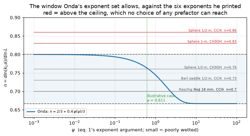
4. The column, and the elasticity of packed height to every printed constant
Onda’s eq. (6) with \(k_G\), \(k_L\) and \(a_w\) from eqs. (1)–(3), solved as a counter-current BVP. The number a designer wants is the packed height \(Z\) for a duty; what this section measures is how much of that height each printed constant is responsible for.
The elasticity \(\partial\ln Z/\partial p\) is available analytically, because at fixed duty \(Z \propto R_G + R_L\) and the chain rule collapses onto two numbers, the gas-side resistance fraction \(f_G\) and the wetting function \(\varphi(\psi)\):
\[\frac{\partial\ln Z}{\partial \ln C_{k_G}} = -f_G,\qquad \frac{\partial\ln Z}{\partial \ln C_{k_L}} = -f_L,\qquad \frac{\partial\ln Z}{\partial \ln C_{a_w}} = -\Bigl(f_G+\tfrac{f_L}{3}\Bigr)\varphi,\]
and for each exponent \(e\) multiplying a group \(\Pi\), the semi-elasticity is the same coefficient times \(\ln\Pi\). The \(f_L/3\) rather than \(f_L\) is the coupling: raising \(a_w\) raises the area but lowers \(k_L\) through \(Re_{L,w}\), and \(1-2/3=1/3\) of the gain survives.
Those analytic elasticities are then checked against central finite differences on \(Z\), a route that shares no algebra with them, and the finite-difference route is then re-run through the pymrm column solve itself, so the check reaches the operator assembly and not only the resistance arithmetic.
M_SLOPE = 1.0          # straight equilibrium line y* = m x; a page parameter
Y_IN, X_IN = 0.02, 0.0
REMOVAL = 0.95
N_CELLS = 200

def height_for_duty(o, *, m=M_SLOPE, L=L_REF, G=G_REF, removal=REMOVAL):
    """Packed height for a stated removal, from the closed form of the same BVP."""
    KGa = o.KGa(L, G, m, C_AV)
    f = lambda Z: column_closed_form(Z, KGa, m, G_M, L_M, Y_IN, X_IN)[0] - (1 - removal) * Y_IN
    return one_root(f, 1e-4, 500.0, "packed height for the duty", log=True), KGa

Z_STAR, KGA_REF = height_for_duty(onda)
F_G_REF = onda.f_G(L_REF, G_REF, M_SLOPE, C_AV)
PHI_REF = float(onda.phi(L_REF))
ABSORPTION_FACTOR = L_M / (M_SLOPE * G_M)
print(f"duty: {100*REMOVAL:.0f} % removal of a dilute solute, y_in = {Y_IN}, m = {M_SLOPE}")
print(f"   absorption factor L_M/(m G_M) = {ABSORPTION_FACTOR:.3f}   (> 1, so no pinch)")
print(f"   K_G a  = {KGA_REF:.3f} kg-mole/(m3 hr) per unit mole fraction")
print(f"   f_G    = {F_G_REF:.4f}   (gas-side share of the total resistance)")
print(f"   phi    = {PHI_REF:.4f}   (wetting function at psi = {PSI_REF:.4f})")
print(f"   Z*     = {Z_STAR:.5f} m of packing")

col = Absorber(Z_STAR, KGA_REF, M_SLOPE, G_M, L_M, Y_IN, X_IN, n=N_CELLS).solve()
col_dc = Absorber(Z_STAR, KGA_REF, M_SLOPE, G_M, L_M, Y_IN, X_IN, n=N_CELLS).solve(route="deferred")
Y_EXACT, X_EXACT = column_closed_form(Z_STAR, KGA_REF, M_SLOPE, G_M, L_M, Y_IN, X_IN)
COL_ROUTES_GAP = float(np.abs(col.u - col_dc.u).max() / np.abs(col.u).max())
print(f"\npymrm column at n = {N_CELLS}: Newton on the exact van Leer Jacobian, {col.its} "
      f"iterations;")
print(f"   deferred correction on the factorised upwind matrix, {col_dc.its} back-substitutions;")
print(f"   the two fields agree {'below' if COL_ROUTES_GAP < 1e-10 else 'ABOVE'} 1e-10 of the "
      "largest mole fraction")
print(f"   y_out  = {col.y_out:.8e}   closed form {Y_EXACT:.8e}")
print(f"   x_out  = {col.x_out:.8e}   closed form {X_EXACT:.8e}")
print(f"   solute balance, gas lost vs liquid gained: {col.imbalance():.3e} relative")
COL_IMBALANCE = float(col.imbalance())
duty: 95 % removal of a dilute solute, y_in = 0.02, m = 1.0
absorption factor L_M/(m G_M) = 6.430 (> 1, so no pinch)
K_G a = 287.631 kg-mole/(m3 hr) per unit mole fraction
f_G = 0.7497 (gas-side share of the total resistance)
phi = 0.7254 (wetting function at psi = 0.6111)
Z* = 0.80629 m of packing
pymrm column at n = 200: Newton on the exact van Leer Jacobian, 5 iterations;
deferred correction on the factorised upwind matrix, 29 back-substitutions;
the two fields agree below 1e-10 of the largest mole fraction
y_out = 1.00003013e-03 closed form 1.00000000e-03
x_out = 2.95480367e-03 closed form 2.95480836e-03
solute balance, gas lost vs liquid gained: 2.220e-16 relativefig, ax = plt.subplots(1, 2, figsize=(10.4, 3.8))
zz = np.linspace(0, Z_STAR, 400)
lam = KGA_REF * (1 / G_M - M_SLOPE / L_M)
E_ = np.exp(-lam * Z_STAR); beta_ = (M_SLOPE * KGA_REF / L_M) / lam
D0_ = (Y_IN - M_SLOPE * X_IN) / (1 + beta_ * (1 - E_))
y_ex = Y_IN - (KGA_REF / G_M) * D0_ * (1 - np.exp(-lam * zz)) / lam
x_ex = X_IN + (KGA_REF / L_M) * D0_ * (np.exp(-lam * zz) - np.exp(-lam * Z_STAR)) / lam
ax[0].plot(zz, 1e3 * y_ex, "-", lw=1.6, color="0.4", label="closed form")
ax[0].plot(col.z_c.ravel(), 1e3 * col.u[:, 0], "o", ms=3, mfc="none", color="C0",
label=f"pymrm, n = {N_CELLS}")
ax[0].set_xlabel("z from the bottom / m"); ax[0].set_ylabel(r"$y \times 10^{3}$")
ax[0].set_title("gas, rising"); ax[0].legend(fontsize=8)
ax[1].plot(zz, 1e3 * x_ex, "-", lw=1.6, color="0.4", label="closed form")
ax[1].plot(col.z_c.ravel(), 1e3 * col.u[:, 1], "s", ms=3, mfc="none", color="C3",
label=f"pymrm, n = {N_CELLS}")
ax[1].set_xlabel("z from the bottom / m"); ax[1].set_ylabel(r"$x \times 10^{3}$")
ax[1].set_title("liquid, falling"); ax[1].legend(fontsize=8)
fig.suptitle(f"Onda's eq. (6) as a counter-current BVP: {100*REMOVAL:.0f} % removal "
f"in {Z_STAR:.3f} m of 1-in spheres", fontsize=10)
fig.tight_layout(); plt.show()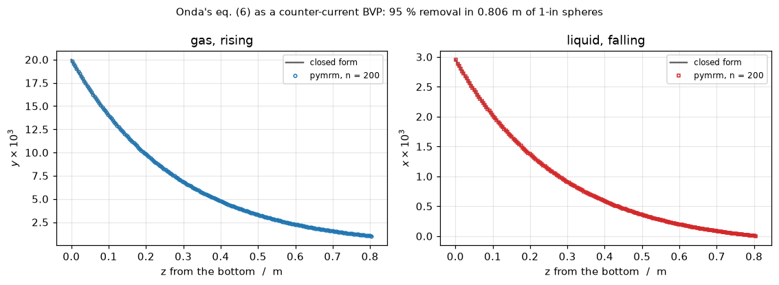
# ---- analytic elasticities ------------------------------------------------
def groups_at(o, L, G):
    return dict(
        e_sigma=np.log(o.sigma_ratio),
        e_Re_L=np.log(L / (o.a_t * o.mu_L)),
        e_Fr_L=np.log(L**2 * o.a_t / (o.rho_L**2 * G_ACC)),
        e_We_L=np.log(L**2 / (o.rho_L * o.sigma * o.a_t)),
        e_Re_Lw=np.log(L / (o.a_w(L) * o.mu_L)),
        e_Sc_L=np.log(o.Sc_L),
        e_atDp_L=np.log(o.atDp),
        e_Re_G=np.log(G / (o.a_t * o.mu_G)),
        e_Sc_G=np.log(o.Sc_G),
        e_atDp_G=np.log(o.atDp),
    )

def elasticities_analytic(o, L, G, m):
    fG = o.f_G(L, G, m, C_AV); fL = 1 - fG; ph = o.phi(L)
    kA = -(fG + fL * (1 - E_RE_LW))          # dlnZ / dln(a_w)
    g = groups_at(o, L, G)
    out = {"C_aw": kA * ph, "C_kL": -fL, "C_kG": -fG}
    for e in ("e_sigma", "e_Re_L", "e_Fr_L", "e_We_L"):
        out[e] = kA * ph * g[e]                      # via a_w
    for e in ("e_Re_Lw", "e_Sc_L", "e_atDp_L"):
        out[e] = -fL * g[e]                          # via k_L
    for e in ("e_Re_G", "e_Sc_G", "e_atDp_G"):
        out[e] = -fG * g[e]                          # via k_G
    return out

# ---- numeric elasticities: central differences on the SOLVED column -------
BASE = dict(C_aw=C_AW, e_sigma=E_SIG, e_Re_L=E_RE_L, e_Fr_L=E_FR_L, e_We_L=E_WE_L,
            C_kL=C_KL, e_Re_Lw=E_RE_LW, e_Sc_L=E_SC_L, e_atDp_L=E_ATDP_L,
            C_kG=C_KG, e_Re_G=E_RE_G, e_Sc_G=E_SC_G, e_atDp_G=E_ATDP_G)

def onda_with(**over):
    kw = dict(BASE); kw.update(over)
    return OndaSet(a_t=A_T, D_p=D_P, sigma_ratio=SIGMA_RATIO, **PROPS, **kw)

def elasticity_numeric(name, h=1e-4, m=M_SLOPE, L=L_REF, G=G_REF):
    """dlnZ/dln(param) for a prefactor, dlnZ/d(param) for an exponent.

    Z comes from a root find on the CLOSED FORM; the cell below confirms the
    pymrm column reproduces the same Z, so the two agree on what is being
    differentiated.
    """
    v0 = BASE[name]
    if name.startswith("C_"):
        lo, hi = v0 * (1 - h), v0 * (1 + h); dlnp = np.log(hi / lo)
    else:
        lo, hi = v0 - h, v0 + h; dlnp = hi - lo
    Zlo = height_for_duty(onda_with(**{name: lo}), m=m, L=L, G=G)[0]
    Zhi = height_for_duty(onda_with(**{name: hi}), m=m, L=L, G=G)[0]
    return (np.log(Zhi) - np.log(Zlo)) / dlnp

ana = elasticities_analytic(onda, L_REF, G_REF, M_SLOPE)
rows = []
for name in BASE:
    a_, n_ = ana[name], elasticity_numeric(name)
    rows.append((name, float(K.loc[K.symbol == name, "value"].iloc[0]),
                 a_, n_, abs(a_ - n_)))
el = pd.DataFrame(rows, columns=["printed constant", "value",
                                 "elasticity, analytic (chain rule)",
                                 "elasticity, finite difference on Z",
                                 "|difference|"])
el["|elasticity|"] = el["elasticity, analytic (chain rule)"].abs()
el = el.sort_values("|elasticity|", ascending=False)
display(el.drop(columns="|elasticity|").round(6))
ELASTICITY_TWO_ROUTES = float(el["|difference|"].max())
print(f"analytic chain rule vs finite differences on Z: worst "
      f"{ELASTICITY_TWO_ROUTES:.3e}")
print(f"\nSum rule: the three PREFACTOR elasticities must satisfy")
print(f"   -(C_kG) - (C_kL) = f_G + f_L = 1 exactly, by construction.")
SUM_RULE = abs(-(ana["C_kG"] + ana["C_kL"]) - 1.0)
print(f"   residual {SUM_RULE:.2e}   <- structural, cannot fail; reported as an identity")
EL_MAX = float(el["|elasticity|"].max())
EL_MIN = float(el["|elasticity|"].min())
EL_ARGMIN = str(el.iloc[-1]["printed constant"])    # the table row with the smallest |elasticity|
print(f"\nlargest  |elasticity|: {EL_MAX:.4f}  ({el.iloc[0]['printed constant']})")
print(f"smallest |elasticity|: {EL_MIN:.4g}  ({EL_ARGMIN})")
print(f"\nTHE SECOND NEARLY-INERT EXPONENT. eq. (3)'s Schmidt exponent 1/3 has")
print(f"semi-elasticity -f_G ln(Sc_G) = {ana['e_Sc_G']:+.5f}, because Sc_G = "
      f"{onda.Sc_G:.4f} for this")
print(f"gas and ln(Sc_G) = {np.log(onda.Sc_G):+.5f} is nearly zero. Replacing 1/3 by 2/3")
_o23 = onda_with(e_Sc_G=2 * E_SC_G)
E_SCG_2X_RELDEV = abs(height_for_duty(_o23)[0] / Z_STAR - 1.0)
print(f"moves the packed height by {100*E_SCG_2X_RELDEV:.3f} %. Almost every gas of")
print("industrial interest has Sc_G within a factor two of 1, so a design")
print("calculation essentially cannot see this exponent - which is precisely why")
print("the eq. (4) identity, where it shows up STRUCTURALLY through the Schmidt")
print("cancellation rather than numerically, is the check that pins it.")| printed constant | value | elasticity, analytic (chain rule) | elasticity, finite difference on Z | |difference| | |
|---|---|---|---|---|---|
| 3 | e_Fr_L | -0.050000 | 5.800997 | 5.800996 | 0.0 |
| 4 | e_We_L | 0.200000 | 4.576987 | 4.576987 | 0.0 |
| 10 | e_Re_G | 0.700000 | -4.062499 | -4.062499 | 0.0 |
| 2 | e_Re_L | 0.100000 | -1.768332 | -1.768332 | 0.0 |
| 7 | e_Sc_L | -0.500000 | -1.537113 | -1.537113 | 0.0 |
| 6 | e_Re_Lw | 0.666667 | -0.928122 | -0.928122 | 0.0 |
| 12 | e_atDp_G | -2.000000 | -0.917505 | -0.917505 | 0.0 |
| 9 | C_kG | 5.230000 | -0.749733 | -0.749733 | 0.0 |
| 0 | C_aw | 1.450000 | -0.604348 | -0.604348 | 0.0 |
| 8 | e_atDp_L | 0.400000 | -0.306270 | -0.306270 | 0.0 |
| 5 | C_kL | 0.005100 | -0.250267 | -0.250267 | 0.0 |
| 1 | e_sigma | 0.750000 | 0.098218 | 0.098218 | 0.0 |
| 11 | e_Sc_G | 0.333333 | 0.021845 | 0.021845 | 0.0 |
analytic chain rule vs finite differences on Z: worst 1.764e-07

Sum rule: the three PREFACTOR elasticities must satisfy
   -(C_kG) - (C_kL) = f_G + f_L = 1 exactly, by construction.
   residual 0.00e+00   <- structural, cannot fail; reported as an identity

largest  |elasticity|: 5.8010  (e_Fr_L)
smallest |elasticity|: 0.02184  (e_Sc_G)

THE SECOND NEARLY-INERT EXPONENT. eq. (3)'s Schmidt exponent 1/3 has
semi-elasticity -f_G ln(Sc_G) = +0.02184, because Sc_G = 0.9713 for this
gas and ln(Sc_G) = -0.02914 is nearly zero. Replacing 1/3 by 2/3
moves the packed height by 0.732 %. Almost every gas of
industrial interest has Sc_G within a factor two of 1, so a design
calculation essentially cannot see this exponent - which is precisely why
the eq. (4) identity, where it shows up STRUCTURALLY through the Schmidt
cancellation rather than numerically, is the check that pins it.
And the same three prefactor elasticities, re-measured through the pymrm solve. The finite differences above are on \(Z\) from the closed form, which shares the resistance arithmetic with the analytic route but not its chain rule. Pushing the same perturbation through the column solve closes the last gap: it exercises the operator assembly, the boundary conditions and the Newton solve as well. At fixed \(Z\) the quantity differentiated is \(\ln y_{out}\) rather than \(\ln Z\), and the two are related by the same \(\mathrm{d}\ln y_{out}/\mathrm{d}\ln K_Ga\) for every parameter, so dividing one by the other recovers the elasticity of \(Z\) with no further algebra, and the agreement is limited only by the column’s own discretisation error.
def dlogy_dlogp_column(name, h=1e-3, n=400):
    """d ln(y_out)/d ln(param) measured on the SOLVED pymrm column, at fixed Z."""
    v0 = BASE[name]; lo, hi = v0 * (1 - h), v0 * (1 + h)
    out = []
    for v in (lo, hi):
        o = onda_with(**{name: v})
        cc = Absorber(Z_STAR, o.KGa(L_REF, G_REF, M_SLOPE, C_AV), M_SLOPE,
                      G_M, L_M, Y_IN, X_IN, n=n).solve()
        out.append(np.log(cc.y_out))
    return (out[1] - out[0]) / np.log(hi / lo)

# the normaliser: d ln(y_out)/d ln(K_G a), measured the same way
cc_lo = Absorber(Z_STAR, KGA_REF * 0.999, M_SLOPE, G_M, L_M, Y_IN, X_IN, n=400).solve()
cc_hi = Absorber(Z_STAR, KGA_REF * 1.001, M_SLOPE, G_M, L_M, Y_IN, X_IN, n=400).solve()
DLOGY_DLOGK = (np.log(cc_hi.y_out) - np.log(cc_lo.y_out)) / np.log(1.001 / 0.999)

rows = []
for name in ("C_kG", "C_kL", "C_aw"):
    col_el = -dlogy_dlogp_column(name) / DLOGY_DLOGK      # dlnZ/dlnp = -dlny/dlnp / (dlny/dlnK)
    rows.append((name, ana[name], elasticity_numeric(name), col_el,
                 abs(col_el - ana[name])))
elc = pd.DataFrame(rows, columns=["prefactor", "analytic (chain rule)",
                                  "finite difference on Z",
                                  "through the pymrm column solve", "|column - analytic|"])
display(elc.round(8))
ELASTICITY_COLUMN_ROUTE = float(elc["|column - analytic|"].max())
print(f"d ln(y_out)/d ln(K_G a) on the column = {DLOGY_DLOGK:.6f}")
print(f"worst disagreement between the analytic chain rule and the column route: "
      f"{ELASTICITY_COLUMN_ROUTE:.2e}")
print("That floor is the column's own discretisation error at n = 400, not an")
print("error in either derivation - the closed-form route agrees to "
f"{ELASTICITY_TWO_ROUTES:.1e}.")| prefactor | analytic (chain rule) | finite difference on Z | through the pymrm column solve | |column - analytic| | |
|---|---|---|---|---|---|
| 0 | C_kG | -0.749733 | -0.749733 | -0.749733 | 5.000000e-08 |
| 1 | C_kL | -0.250267 | -0.250267 | -0.250267 | 1.400000e-07 |
| 2 | C_aw | -0.604348 | -0.604348 | -0.604348 | 8.000000e-08 |
d ln(y_out)/d ln(K_G a) on the column = -2.861976
worst disagreement between the analytic chain rule and the column route: 1.39e-07
That floor is the column's own discretisation error at n = 400, not an
error in either derivation - the closed-form route agrees to 1.8e-07.
One constant is exactly inert, and it is not an accident of the operating point. The semi-elasticity of \(Z\) to the exponent 0.75 is proportional to \(\ln(\sigma_c/\sigma)\). When the packing’s critical surface tension equals the liquid’s, that logarithm is zero and the exponent 0.75 can be set to any value whatever without moving anything, it is not merely small, it is identically zero: a term that is provably inert for a whole class of callers, and it needs saying, because \(\sigma_c \approx \sigma\) is not exotic (it is roughly the ceramic/water case).
The cell below demonstrates it rather than asserting it: with \(\sigma_c/\sigma = 1\), replacing 0.75 by 7.5 leaves every digit of \(Z\).
o_eq = OndaSet(a_t=A_T, D_p=D_P, sigma_ratio=1.0, **PROPS)
Z_eq, _ = height_for_duty(o_eq)
o_eq_bad = OndaSet(a_t=A_T, D_p=D_P, sigma_ratio=1.0, **PROPS, e_sigma=10 * E_SIG)
Z_eq_bad, _ = height_for_duty(o_eq_bad)
INERT_075_RELDEV = abs(Z_eq_bad / Z_eq - 1.0)
print(f"at sigma_c/sigma = 1.0:   e_sigma = {E_SIG} -> Z = {Z_eq:.12f} m")
print(f"                          e_sigma = {10*E_SIG}  -> Z = {Z_eq_bad:.12f} m")
print(f"   relative change: {INERT_075_RELDEV:.3e}   <- exactly inert, not merely small")

o_ne = OndaSet(a_t=A_T, D_p=D_P, sigma_ratio=SIGMA_RATIO, **PROPS)
o_ne_bad = OndaSet(a_t=A_T, D_p=D_P, sigma_ratio=SIGMA_RATIO, **PROPS, e_sigma=10 * E_SIG)
Z_ne, _ = height_for_duty(o_ne); Z_ne_bad, _ = height_for_duty(o_ne_bad)
LIVE_075_RELDEV = abs(Z_ne_bad / Z_ne - 1.0)
print(f"\nat sigma_c/sigma = {SIGMA_RATIO}:  the same substitution moves Z by "
      f"{100*LIVE_075_RELDEV:.2f} %")
print("So 0.75 is live only when the packing and the liquid differ in surface")
print("tension, and this ARTICLE prints no sigma_c for any material - it is in ref. 18.")
at sigma_c/sigma = 1.0: e_sigma = 0.75 -> Z = 0.750433059824 m
e_sigma = 7.5 -> Z = 0.750433059824 m
relative change: 0.000e+00 <- exactly inert, not merely small
at sigma_c/sigma = 0.85: the same substitution moves Z by 119.61 %
So 0.75 is live only when the packing and the liquid differ in surface
tension, and this ARTICLE prints no sigma_c for any material - it is in ref. 18.sr = np.linspace(0.5, 1.5, 21)
Zs, aws, els = [], [], []
for r_ in sr:
o = OndaSet(a_t=A_T, D_p=D_P, sigma_ratio=r_, **PROPS)
Zs.append(height_for_duty(o)[0]); aws.append(o.a_w(L_REF) / A_T)
els.append(elasticities_analytic(o, L_REF, G_REF, M_SLOPE)["e_sigma"])
Zs, aws, els = map(np.array, (Zs, aws, els))
SIGMA_SWEEP_Z_FACTOR = float(Zs.max() / Zs.min())
SIGMA_SWEEP_AW_LO, SIGMA_SWEEP_AW_HI = float(aws.min()), float(aws.max())
print("sigma_c/sigma swept over 0.5 .. 1.5 (the page parameter this article cannot supply):")
print(f" a_w/a_t {SIGMA_SWEEP_AW_LO:.4f} .. {SIGMA_SWEEP_AW_HI:.4f}")
print(f" Z {Zs.max():.4f} .. {Zs.min():.4f} m, a factor {SIGMA_SWEEP_Z_FACTOR:.3f}")
print(f" semi-elasticity of Z to the exponent 0.75 changes SIGN at sigma_c/sigma = 1:")
print(f" at 0.5 {els[0]:+.4f} at 1.0 {els[len(sr)//2]+0.0:+.1e} "
f"at 1.5 {els[-1]:+.4f}")
fig, ax = plt.subplots(1, 2, figsize=(10.2, 3.6))
ax[0].plot(sr, aws, "-", lw=1.8, color="C0"); ax[0].set_ylabel(r"$a_w/a_t$")
ax[1].plot(sr, els, "-", lw=1.8, color="C3"); ax[1].axhline(0, color="0.4", lw=1)
ax[1].set_ylabel(r"$\partial\ln Z/\partial e_\sigma$")
for a_ in ax:
a_.axvline(1.0, ls=":", color="0.5", lw=1.2); a_.set_xlabel(r"$\sigma_c/\sigma$")
ax[0].set_title("wetted fraction"); ax[1].set_title("the 0.75 is inert exactly at 1.0")
fig.tight_layout(); plt.show()sigma_c/sigma swept over 0.5 .. 1.5 (the page parameter this article cannot supply):
a_w/a_t 0.3367 .. 0.6077
Z 1.0445 .. 0.6384 m, a factor 1.636
semi-elasticity of Z to the exponent 0.75 changes SIGN at sigma_c/sigma = 1:
at 0.5 +0.4806 at 1.0 +0.0e+00 at 1.5 -0.1980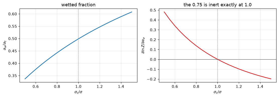
5. Where each correlation is live: sweeping the equilibrium slope
Onda’s Fig. 9 makes the same point for distillation. Here the resistance split is swept over four decades of \(m\) at fixed hydraulics, which is what says where eq. (2) and eq. (3) each matter, and therefore where a mis-set constant in either would be felt and where it would not.
Only part of this range has a column that meets the duty. A counter-current column fed solute-free liquid removes at most the fraction \(L_M/(mG_M)\) of the solute however tall it is, so a packed height that meets the duty exists only up to the slope where that limit falls to the duty (found as a root further down). The sweep of the resistance split needs no column and runs over the whole range; the height is reported only where one exists.
ms = np.logspace(-1, np.log10(2000.0), 400)
fG = np.array([onda.f_G(L_REF, G_REF, m, C_AV) for m in ms])
M_PINCH = L_M / G_M
F_G_AT_MIN_M, F_G_AT_MAX_M = float(fG[0]), float(fG[-1])
M_HALF = one_root(lambda m: onda.f_G(L_REF, G_REF, m, C_AV) - 0.5, 1e-3, 1e4,
                  "equal resistances", log=True)
print(f"gas-side resistance share f_G over m = {ms[0]:g} .. {ms[-1]:g}:")
print(f"   {F_G_AT_MIN_M:.4f} down to {F_G_AT_MAX_M:.5f}")
print(f"   50/50 split at m = {M_HALF:.4f}")
print(f"   absorption factor reaches 1 at m = L_M/G_M = {M_PINCH:.3f}")
print(f"   up to there, f_G runs "
      f"{onda.f_G(L_REF,G_REF,ms[0],C_AV):.4f} .. {onda.f_G(L_REF,G_REF,0.99*M_PINCH,C_AV):.4f}")

fig, ax = plt.subplots(figsize=(7.4, 4.0))
ax.semilogx(ms, fG, "-", lw=2, color="C0")
ax.axvline(M_PINCH, ls="--", color="C3", lw=1.2)
ax.axvline(M_HALF, ls=":", color="0.5", lw=1.2)
ax.fill_between(ms, 0, 1, where=(ms > M_PINCH), color="C3", alpha=0.06)
ax.annotate(f"absorption factor below 1\nbeyond m = {M_PINCH:.2f}\n"
            "at this L/G", (M_PINCH * 1.3, 0.55), fontsize=8, color="C3")
ax.annotate(f"50/50 at m = {M_HALF:.2f}", (M_HALF, 0.5), textcoords="offset points",
            xytext=(-100, 6), fontsize=8, color="0.3")
ax.set_xlabel("m, slope of the equilibrium line")
ax.set_ylabel(r"$f_G$ = gas-side share of $1/K_Ga$")
ax.set_ylim(0, 1)
ax.set_title("Which of Onda's three equations a design calculation can feel\n"
             r"$f_G\to1$: only eq. (3) matters.  $f_G\to0$: only eqs. (1) and (2) matter.")
fig.tight_layout(); plt.show()
gas-side resistance share f_G over m = 0.1 .. 2000:
0.9677 down to 0.00150
50/50 split at m = 2.9957
absorption factor reaches 1 at m = L_M/G_M = 6.430
up to there, f_G runs 0.9677 .. 0.3200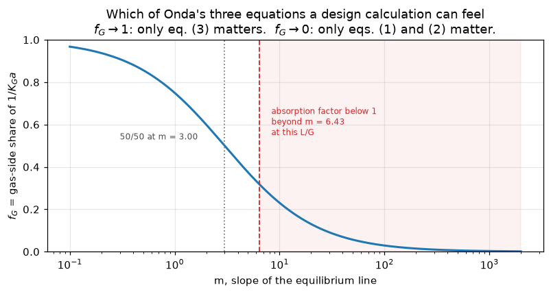
6. The branch: 5.23 against 2.00
Eq. (3)’s prefactor is branched, and a branched correlation is exactly where a page can test only one branch without noticing, and then the other branch’s constant is never read. So both branches are run here, at the geometry the paper itself assigns to the lower one.
The paper’s criterion, stated three times: “Raschig rings and Berl saddles smaller than 15 mm” (page 58), “Raschig rings smaller than 15 mm and Berl saddles smaller than 1/2”“ (page 61), and for vaporization “for 1/2-in. sphere the constant of Eq.(3) might be changed into 2.00” (page 60). Half-inch spheres are therefore the one geometry for which this article explicitly names the lower branch and supplies \(a_t D_p\), so they are what is used.
BRANCH_FACTOR = C_KG / C_KG_SMALL
D_P_SMALL = 0.0127                      # 1/2-in spheres: the paper's own branch example
A_T_SMALL = ATDP_SPHERES / D_P_SMALL
rows = []
for label, dp, at_, Ck in [("1-in spheres, upper branch", D_P, A_T, C_KG),
                           ("1/2-in spheres, upper branch", D_P_SMALL, A_T_SMALL, C_KG),
                           ("1/2-in spheres, LOWER branch", D_P_SMALL, A_T_SMALL, C_KG_SMALL)]:
    o = OndaSet(a_t=at_, D_p=dp, sigma_ratio=SIGMA_RATIO, **PROPS, C_kG=Ck)
    Z, KGa = height_for_duty(o)
    rows.append((label, Ck, o.k_G(G_REF), o.f_G(L_REF, G_REF, M_SLOPE, C_AV), KGa, Z))
br = pd.DataFrame(rows, columns=["case", "eq. (3) prefactor", "k_G", "f_G", "K_G a", "Z / m"])
display(br.round(5))
Z_UPPER_SMALL = float(br.loc[1, "Z / m"]); Z_LOWER_SMALL = float(br.loc[2, "Z / m"])
BRANCH_Z_FACTOR = Z_LOWER_SMALL / Z_UPPER_SMALL
print(f"branch factor on the constant itself: {C_KG}/{C_KG_SMALL} = {BRANCH_FACTOR:.4f}")
print(f"branch factor on the PACKED HEIGHT for the same duty: {BRANCH_Z_FACTOR:.4f}")
print(f"   ({Z_UPPER_SMALL:.4f} m -> {Z_LOWER_SMALL:.4f} m)")
print("The height factor is smaller than the constant factor because the liquid")
print(f"film carries {100*(1-float(br.loc[1,'f_G'])):.1f} % of the resistance here and does not move.")
print("On a gas-film-controlled duty the two factors would coincide; that is the")
print("reason the branch is reported as a height, not as a coefficient ratio.")| case | eq. (3) prefactor | k_G | f_G | K_G a | Z / m | |
|---|---|---|---|---|---|---|
| 0 | 1-in spheres, upper branch | 5.23 | 6.26796 | 0.74973 | 287.63111 | 0.80629 |
| 1 | 1/2-in spheres, upper branch | 5.23 | 7.71676 | 0.63390 | 498.80057 | 0.46494 |
| 2 | 1/2-in spheres, LOWER branch | 2.00 | 2.95096 | 0.81910 | 246.47430 | 0.94092 |
branch factor on the constant itself: 5.23/2.0 = 2.6150
branch factor on the PACKED HEIGHT for the same duty: 2.0237
   (0.4649 m -> 0.9409 m)
The height factor is smaller than the constant factor because the liquid
film carries 36.6 % of the resistance here and does not move.
On a gas-film-controlled duty the two factors would coincide; that is the
reason the branch is reported as a height, not as a coefficient ratio.Validation
Four checks, ranked by what they can catch, plus a statement of what none of them can.
V1: the eq. (4) identity, two independent routes. Route A is symbolic; Route B evaluates eq. (3) numerically at four thousand random property combinations and regresses, doing no algebra at all. It is the only check that pins all four gas-side constants at once.
V2: eq. (4) against Shulman’s eq. (5). Two correlations fitted to disjoint experiments; the paper claims “fairly good” and the page puts a number on it.
V3: the exponent window against Table 1. In-sample, with two rows above the ceiling.
V4: the pymrm column against the closed form of the same BVP. A discretisation check and nothing more.
The elasticity table is a two-route check as well: the analytic chain rule against central differences on \(Z\), and against the same differences pushed through the column solve. It fails if either the derivation or OndaSet is wrong.
V4: what the column check is, and what it is not
A ladder of six nested grids, 25 to 800 cells. Orders come from successive differences of the outlet value, so no exact value enters them; the closed form is compared only with the outlet value at the finest grid and with the Richardson limit of the ladder. The round-off companion divides the finest successive difference by the larger of the solver’s stopping tolerance and the measured gap between the two solver routes. The same ladder is read a second way, at the centre of the last cell instead of the outlet face, to measure what that reading costs.
NS = (25, 50, 100, 200, 400, 800)


def col_study(ns=NS, scheme="vanleer", rtol=1e-12, dc_rtol=1e-12, cocurrent=False,
              read="face", n_shift=N_CELLS, limiter=vanleer):
    """Grid ladder of the column at the design point; every column claim, by name."""
    cols, gap = {}, 0.0
    for n in ns:
        mk = lambda: Absorber(Z_STAR, KGA_REF, M_SLOPE, G_M, L_M, Y_IN, X_IN, n=n, limiter=limiter,
                              cocurrent=cocurrent)
        c = mk().solve(scheme, rtol=rtol)
        if scheme == "vanleer":
            try:                                  # the second route, deferred correction
                d = mk().solve(route="deferred", rtol=dc_rtol)
                gap = max(gap, float(np.abs(c.u - d.u).max() / np.abs(c.u).max()))
            except RuntimeError:                  # it may stall (pitfall P10): no gap then
                gap = np.nan
        cols[n] = c
    y = (lambda n: cols[n].y_out_cell) if read == "cell" else (lambda n: cols[n].y_out)
    face = observed_orders(y, ns)
    cell = observed_orders(lambda n: cols[n].y_out_cell, ns)
    fin = cols[ns[-1]]
    vals = np.array([y(n) for n in ns])
    floor = np.nanmax([gap, rtol]) * np.abs(fin.u).max()
    shift = Absorber(Z_STAR, KGA_REF, M_SLOPE, G_M, L_M, Y_IN, X_IN, n=n_shift,
                     limiter=limiter, cocurrent=cocurrent).solve(scheme)
    return dict(
        ladder=pd.DataFrame({"n": ns, "y_out, face": [cols[n].y_out for n in ns],
                             "y_out, last cell": [cols[n].y_out_cell for n in ns],
                             "iterations": [cols[n].its for n in ns]}),
        face_orders=face["orders"], cell_orders=cell["orders"],
        col_order_face_min=float(np.min(face["orders"])),
        col_order_face_max=float(np.max(face["orders"])),
        col_ladder_over_roundoff=float(np.min(np.abs(np.diff(vals))) / floor),
        col_richardson_reldev=abs(float(face["extrapolated"]) / Y_EXACT - 1.0),
        col_raw_reldev=abs(y(ns[-1]) / Y_EXACT - 1.0),
        col_imbalance=fin.imbalance(cell=(read == "cell")),
        col_routes_gap=gap,
        col_order_cell_finest=float(cell["orders"][-1]),
        col_cell_centre_reldev=abs(fin.y_out_cell / Y_EXACT - 1.0),
        col_cell_imbalance=fin.imbalance(cell=True),
        col_half_cell_shift=abs(shift.y_out_cell / shift.y_out - 1.0))


COL = col_study()
display(COL["ladder"])
print("observed orders, successive differences of the outlet FACE value: "
      + ", ".join(f"{p:.4f}" for p in COL["face_orders"]))
print("the same ladder read at the LAST CELL CENTRE:                    "
      + ", ".join(f"{p:.4f}" for p in COL["cell_orders"]))
print(f"finest successive difference over the round-off floor: {COL['col_ladder_over_roundoff']:.2e}")
print("Newton against deferred correction, worst over the ladder: below 1e-10 "
      "of the largest mole fraction")
print(f"\nagainst the closed form at n = {NS[-1]}:  face {COL['col_raw_reldev']:.3e}   "
      f"last cell {COL['col_cell_centre_reldev']:.3e}   "
      f"({COL['col_cell_centre_reldev'] / COL['col_raw_reldev']:.0f} times larger)")
print(f"Richardson limit of the face ladder against the closed form: "
      f"{COL['col_richardson_reldev']:.2e}")
print(f"solute balance at n = {NS[-1]}: face values below 1e-13, "
      f"last-cell values {COL['col_cell_imbalance']:.2e}")
print(f"\nReading the outlet at the centre of the last cell instead of at the face costs "
      f"{100 * COL['col_half_cell_shift']:.3f} % at n = {N_CELLS}")
print("and turns a second-order outlet value into a first-order one, while every grid")
print("still looks monotone. compute_boundary_values reconstructs the face value the")
print("flux operator transported, which is why the face reading also closes the")
print("solute balance and the cell reading does not.")| n | y_out, face | y_out, last cell | iterations | |
|---|---|---|---|---|
| 0 | 25 | 0.001002 | 0.001027 | 5 |
| 1 | 50 | 0.001000 | 0.001012 | 5 |
| 2 | 100 | 0.001000 | 0.001006 | 5 |
| 3 | 200 | 0.001000 | 0.001003 | 5 |
| 4 | 400 | 0.001000 | 0.001001 | 5 |
| 5 | 800 | 0.001000 | 0.001001 | 5 |
observed orders, successive differences of the outlet FACE value: 1.9301, 1.9613, 1.9797, 1.9896
the same ladder read at the LAST CELL CENTRE:                    1.1422, 1.0761, 1.0396, 1.0202
finest successive difference over the round-off floor: 2.84e+05
Newton against deferred correction, worst over the ladder: below 1e-10 of the largest mole fraction

against the closed form at n = 800:  face 1.901e-06   last cell 7.292e-04   (384 times larger)
Richardson limit of the face ladder against the closed form: 1.04e-08
solute balance at n = 800: face values below 1e-13, last-cell values 6.11e-04

Reading the outlet at the centre of the last cell instead of at the face costs 0.293 % at n = 200
and turns a second-order outlet value into a first-order one, while every grid
still looks monotone. compute_boundary_values reconstructs the face value the
flux operator transported, which is why the face reading also closes the
solute balance and the cell reading does not.
Beyond the pinch. The absorption factor \(A = L_M/(mG_M)\) falls below 1 at \(m = L_M/G_M\). The column at a fixed height still has a solution there (the problem is linear in \((y, x)\) and the solve converges). What stops existing is a height that meets the duty: with solute-free liquid fed, a column of any height removes at most \(\min(1, A)\), so the duty is reachable up to the slope where \(A\) equals the removal, m_duty_limit, a root of (removal at infinite height) minus the duty, checked against the closed form \(L_M/(\text{removal}\,G_M)\). At \(m = 1.1\,L_M/G_M\) the removal at infinite height is below the duty, which proves that no height exists there; the root search for \(Z\) over 1e-4 to 500 m agrees.
M_BEYOND = 1.1 * M_PINCH


def infinite_height_removal(m, L=L_M, G=G_M, cocurrent=False):
    """Removal of a column of infinite height with solute-free liquid fed."""
    A = L / (m * G)
    return A / (1.0 + A) if cocurrent else min(1.0, A)


def pinch_study(removal=REMOVAL, cocurrent=False, G_removal=G_M):
    """The duty limit in m, and at m = 1.1 L_M/G_M the heights that meet the duty and y_out at Z*.

    ``G_removal`` is the gas flow used by the infinite-height removal only (the closed form
    keeps ``G_M``): one route of the two-route check of ``m_duty_limit``."""
    rem = lambda m: infinite_height_removal(m, G=G_removal, cocurrent=cocurrent)
    m_limit = one_root(lambda m: rem(m) - removal, 1e-3, 1e4, "slope where the duty stops being reachable",
                       log=True)
    closed = L_M * ((1.0 - removal) if cocurrent else 1.0) / (removal * G_M)
    KGa = onda.KGa(L_REF, G_REF, M_BEYOND, C_AV)
    f = lambda Z: (column_closed_form(Z, KGa, M_BEYOND, G_M, L_M, Y_IN, X_IN)[0]
                   - (1 - removal) * Y_IN)
    roots = find_roots(f, 1e-4, 500.0, log=True)["roots"]
    c = Absorber(Z_STAR, KGa, M_BEYOND, G_M, L_M, Y_IN, X_IN, n=N_CELLS,
                 cocurrent=cocurrent).solve()
    return dict(duty_heights_beyond_pinch=len(roots),
                y_out_beyond_pinch_over_y_in=c.y_out / Y_IN,
                m_duty_limit=m_limit, m_duty_limit_closed_form_gap=abs(m_limit - closed) / closed,
                removal_inf_beyond_pinch=rem(M_BEYOND))


PINCH = pinch_study()
print(f"a height meeting {100 * REMOVAL:.0f} % removal exists up to m = {PINCH['m_duty_limit']:.3f} "
      f"(closed form L_M/({REMOVAL} G_M) = {L_M / (REMOVAL * G_M):.3f}); "
      f"L_M/G_M = {M_PINCH:.3f}")
print(f"m = 1.1 L_M/G_M = {M_BEYOND:.3f}, absorption factor {L_M / (M_BEYOND * G_M):.3f}, "
      f"removal at infinite height {PINCH['removal_inf_beyond_pinch']:.6f}:")
print(f"   heights in 1e-4 .. 500 m that meet {100 * REMOVAL:.0f} % removal: "
      f"{PINCH['duty_heights_beyond_pinch']}")
print(f"   the column at Z* = {Z_STAR:.4f} m solves; y_out/y_in = "
      f"{PINCH['y_out_beyond_pinch_over_y_in']:.4f}")
a height meeting 95 % removal exists up to m = 6.769 (closed form L_M/(0.95 G_M) = 6.769); L_M/G_M = 6.430
m = 1.1 L_M/G_M = 7.073, absorption factor 0.909, removal at infinite height 0.909091:
heights in 1e-4 .. 500 m that meet 95 % removal: 0
the column at Z* = 0.8063 m solves; y_out/y_in = 0.4449What V4 cannot detect. The closed form and the pymrm column solve the same equations with the same \(K_G a\); only the numerical method differs. So V4 tests the discretisation, the boundary conditions and the operator assembly, and it is blind to every error in the physics upstream of it. A wrong Onda constant, a wrong resistance addition, a wrong \(c_{av}\): each moves both routes identically.
A break row tests that a check responds, never that a result is correct. The reason to believe the eq. (4) prefactor is that two independent derivations and a separately printed number agree, not that perturbing 5.23 moves it.
Claims
Every number the page states, with how it is checked. Closed-form algebra is held to FIXED; results of root finds and solves to SOLV. Residuals, identities, two-route gaps and orders are bounds with their basis.
FIXED, SOLV = 1e-6, 1e-4
EL_SORTED = el["|elasticity|"].to_numpy()
EL_SMALLEST_MARGIN = float(EL_SORTED[-2] / EL_SORTED[-1] - 1.0)
ATDP_HALFUNIT = 0.05                       # half a unit of the last printed digit of 3.4
JD_ATDP_HALFUNITS = abs(JD_ATDP_FOR_0771 - ATDP_SPHERES) / ATDP_HALFUNIT
E_SCG_OVER_BAND = E_SCG_2X_RELDEV / (stated("err_height_pct") / 100.0)
N_HALFUNIT = 0.005                         # half a unit of Table 1's printed n
_edge = np.minimum(np.abs(n_meas - WINDOW_LO), np.abs(n_meas - WINDOW_HI))


def value(name, x, rtol=FIXED, **kw):
    claims.value(name, x, rtol=rtol, **kw)


def bound(name, x, **kw):
    claims.bound(name, x, **kw)


# --- V1: the eq. (4) identity --------------------------------------------------------
for k in ("jd_prefactor_symbolic", "jd_prefactor_numeric", "jd_prefactor_dev_pct"):
    value(k, JD[k])
bound("jd_exponent_numeric", JD_EXPONENT_NUMERIC, min=E_JD_ONDA - 1e-12, max=E_JD_ONDA + 1e-12,
      basis="identity", note="1 - 0.7 exactly; the regression's round-off")
bound("jd_exponent_dev", JD_EXPONENT_DEV, max=1e-12, basis="identity",
      note="the regression recovers 1 - e_Re_G to round-off")
bound("jd_two_routes_spread", JD_ROUTE_SPREAD, max=1e-12, basis="identity",
      note="both routes reduce the same transcribed eq. (3)")
bound("jd_fit_max_resid", JD_FIT_MAX_RESID, max=1e-12, basis="identity",
      note="ln j_D is linear in ln X only if Sc cancels; least-squares round-off")
claims.exact("jd_sc_cancels", SC_CANCELS, note="neither rho_G nor D_G survives the reduction")
value("jd_atDp_for_printed_0771", JD_ATDP_FOR_0771)
bound("jd_atDp_for_0771_halfunits", JD_ATDP_HALFUNITS, max=1.0, basis="chosen",
      note="a_t D_p reproducing 0.771, in half-units of the printed 3.4: inside its precision")
# --- V2: eq. (4) against eq. (5) -------------------------------------------------------
for k, x in (("eq45_dev_at_X100_pct", EQ45_DEV_LO_PCT), ("eq45_dev_at_X10000_pct", EQ45_DEV_HI_PCT),
             ("eq45_max_dev_pct", EQ45_MAX_DEV_PCT), ("eq45_mean_dev_pct", EQ45_MEAN_DEV_PCT),
             ("eq45_crossover_X", EQ45_CROSSOVER_X)):
    value(k, x)
# --- V3: the window and Table 1 --------------------------------------------------------
value("window_lo", WINDOW_LO)
value("window_hi", WINDOW_HI)
bound("n_window_two_routes", N_WINDOW_TWO_ROUTES, max=1e-8, basis="tolerance",
      note="central difference at relative step 1e-5: truncation and round-off")
bound("window_escape_over_sweep", WINDOW_ESCAPE, max=1e-15, basis="identity", structural=True,
      note="the sweep evaluates the same phi the window is derived from")
claims.exact("table1_n_inside", TABLE1_N_INSIDE, margin=float(_edge.min()), min_margin=N_HALFUNIT,
             note="rows with 2/3 < n <= 0.8; margin the smallest distance to an edge")
claims.count("table1_n_above_ceiling", n_meas, WINDOW_HI, min_margin=N_HALFUNIT, relative=False,
             note="rows above the ceiling; margin absolute, against half a printed unit of n")
for k, x in (("table1_worst_excess", TABLE1_WORST_EXCESS), ("table1_n_range", TABLE1_N_RANGE),
             ("mae_window_ceiling", MAE_WINDOW_TOP), ("mae_null_no_area_coupling", MAE_NULL_23),
             ("mae_null_fitted_constant", MAE_NULL_FITTED)):
    value(k, x)
bound("t_n_above_no_coupling", T_N_ABOVE_NO_COUPLING, min=2.571, basis="chosen",
      note="one-sample t of the six exponents minus 2/3; 2.571 is the two-sided 5 % point "
      "for 5 degrees of freedom")
bound("t_ceiling_vs_no_coupling", T_CEILING_VS_NO_COUPLING, min=-2.0, max=2.0, basis="chosen",
      note="paired gap in |error| over its standard error, six rows: not separated")
bound("t_fitted_vs_ceiling", T_FITTED_VS_CEILING, min=-2.0, max=2.0, basis="chosen",
      note="paired gap in |error| over its standard error, six rows: not separated")
# --- the column and what each constant is worth ------------------------------------------
for k, x in (("Z_star_m", Z_STAR), ("f_G_ref", F_G_REF), ("phi_ref", PHI_REF),
             ("a_w_fraction_ref", AW_FRACTION_REF), ("m_for_equal_resistance", M_HALF),
             ("branch_factor", BRANCH_FACTOR), ("branch_Z_factor", BRANCH_Z_FACTOR),
             ("elasticity_max", EL_MAX), ("live_075_reldev", LIVE_075_RELDEV),
             ("e_ScG_doubled_reldev", E_SCG_2X_RELDEV), ("sigma_sweep_Z_factor", SIGMA_SWEEP_Z_FACTOR),
             ("norman_exponent", NORMAN_EXPONENT)):
    value(k, x)
claims.exact("elasticity_smallest_constant", EL_ARGMIN, margin=EL_SMALLEST_MARGIN, min_margin=0.05,
             note="row of the elasticity table with the smallest |dlnZ/dp|; margin to the next")
bound("elasticity_two_routes", ELASTICITY_TWO_ROUTES, max=1e-6, basis="tolerance",
      note="central differences on Z at relative step 1e-4")
bound("elasticity_column_route", ELASTICITY_COLUMN_ROUTE, max=1e-5, basis="tolerance",
      note="central differences at relative step 1e-3 through the column at 400 cells")
bound("e_ScG_doubled_over_height_band", E_SCG_OVER_BAND, max=0.1, basis="chosen",
      note="Z change from 1/3 -> 2/3 over the paper's own +/-30 % height band: unseen")
bound("inert_075_reldev", INERT_075_RELDEV, max=1e-14, basis="identity",
      note="(sigma_c/sigma)^e is 1 for every e when the ratio is 1")
bound("resistance_sum_rule", SUM_RULE, max=1e-15, basis="identity", structural=True,
      note="f_G + f_L = 1 by definition")
# --- V4: the column's numerics -------------------------------------------------------------
bound("col_order_face_min", COL["col_order_face_min"], min=1.9, basis="theory",
      note="van Leer outlet face value, second order")
bound("col_order_face_max", COL["col_order_face_max"], max=2.1, basis="theory",
      note="van Leer outlet face value, second order")
bound("col_ladder_over_roundoff", COL["col_ladder_over_roundoff"], min=1e3, basis="theory",
      note="finest successive difference over the solver tolerance and the two-route gap")
bound("col_richardson_reldev", COL["col_richardson_reldev"], max=1e-7, basis="theory",
      note="Richardson limit of a second-order ladder; next-order terms")
value("col_raw_reldev", COL["col_raw_reldev"], rtol=SOLV)
bound("col_imbalance", COL["col_imbalance"], max=1e-13, basis="identity",
      note="face fluxes telescope; the gap is round-off")
bound("col_routes_gap", COL["col_routes_gap"], max=1e-10, basis="tolerance",
      note="Newton and deferred correction both stopped at a relative step of 1e-12")
bound("col_order_cell_finest", COL["col_order_cell_finest"], min=0.98, max=1.05, basis="theory",
      note="last cell centre, finest triple: half a cell times the outlet gradient, first "
      "order; the printed ladder falls toward 1 from above")
for k in ("col_cell_centre_reldev", "col_cell_imbalance", "col_half_cell_shift"):
    value(k, COL[k], rtol=SOLV)
claims.exact("duty_heights_beyond_pinch", PINCH["duty_heights_beyond_pinch"],
             note="sign changes of y_out - (1 - removal) y_in over Z in 1e-4..500 m")
value("y_out_beyond_pinch_over_y_in", PINCH["y_out_beyond_pinch_over_y_in"], rtol=SOLV)
value("m_duty_limit", PINCH["m_duty_limit"], rtol=SOLV)
bound("m_duty_limit_closed_form_gap", PINCH["m_duty_limit_closed_form_gap"], max=1e-9, basis="tolerance",
      note="root of (removal at infinite height) minus the duty against L_M/(duty G_M)")
value("removal_inf_beyond_pinch", PINCH["removal_inf_beyond_pinch"])
print(f"{len(claims.metrics)} claims registered")
63 claims registeredThe defect-injection table
Every claim above needs a row that fails its own check. Each row reruns one study with one defect, injected through a call argument or a physical parameter: the eq. (4) reduction, the eq. (4)/(5) comparison, the window and Table 1, the column design (heights, shares, elasticities through both routes), the branch, the column numerics and the pinch. A study that cannot be evaluated under a defect (a crossing that disappears) records nan for its claims, which fails them. Each study run with no defect must return the registered values; the cell checks that before it runs a row.
def jd_study(c4=C_JD_ONDA, **kw):
    out = jd_routes(**kw)
    pre = dict(C=kw.get("C", C_KG), e_Re=kw.get("e_Re", E_RE_G), e_atDp=kw.get("e_atDp", E_ATDP_G))
    atdp = one_root(lambda v: jd_prefactor(atDp=v, **pre) - c4, 0.6, SIX, "a_t D_p for 0.771")
    out["jd_prefactor_dev_pct"] = 100.0 * (out["jd_prefactor_symbolic"] / c4 - 1.0)
    out["jd_atDp_for_printed_0771"] = atdp
    out["jd_atDp_for_0771_halfunits"] = abs(atdp - kw.get("atDp", ATDP_SPHERES)) / ATDP_HALFUNIT
    out["jd_sc_cancels"] = out["sc_cancels"]
    return out


def eq45_study(c4=C_JD_ONDA, e4=E_JD_ONDA, c5=C_JD_SHUL, e5=E_JD_SHUL):
    r = lambda X: eq45_ratio(X, c4, e4, c5, e5)
    lo, hi = 100.0 * (r(XLO) - 1.0), 100.0 * (r(XHI) - 1.0)
    if e4 == e5:
        raise ValueError("equal exponents: the two correlations never cross")
    cross = float(np.exp(np.log(c5 / c4) / (e4 - e5)))
    dev = lambda lnX: abs(r(np.exp(lnX)) - 1.0)
    cuts = [np.log(XLO)] + ([np.log(cross)] if XLO < cross < XHI else []) + [np.log(XHI)]
    mean = sum(quad(dev, a, b, epsabs=0.0, epsrel=1e-12)[0] for a, b in zip(cuts, cuts[1:]))
    return dict(eq45_dev_at_X100_pct=lo, eq45_dev_at_X10000_pct=hi,
                eq45_max_dev_pct=max(abs(lo), abs(hi)), eq45_crossover_X=cross,
                eq45_mean_dev_pct=100.0 * mean / np.log(XHI / XLO))


def window_study(n_table=n_meas, analytic_factor=1.0, **exps):
    o = onda_with(**exps)
    e_lw = o.e_Re_Lw
    comp = o.e_Re_L + 2 * o.e_Fr_L + 2 * o.e_We_L
    lo, hi = e_lw, e_lw + comp * (1.0 - e_lw)
    na_ = np.array([e_lw + analytic_factor * comp * (1.0 - e_lw) * o.phi(L) for L in Ls])
    nb_ = np.array([n_pred_numeric(o, L) for L in Ls])
    best = float(np.median(n_table))
    err = lambda p: float(np.abs(n_table - p).mean())

    def t(a, b):
        d = np.abs(n_table - a) - np.abs(n_table - b)
        with np.errstate(divide="ignore", invalid="ignore"):   # equal gaps: t is infinite
            return float(d.mean() / (d.std(ddof=1) / np.sqrt(d.size)))
    return dict(window_lo=lo, window_hi=hi, n_window_two_routes=float(np.abs(na_ - nb_).max()),
                table1_n_inside=int(((n_table > lo) & (n_table <= hi)).sum()),
                table1_n_above_ceiling=int((n_table > hi).sum()),
                table1_worst_excess=float(np.maximum(0.0, n_table - hi).max()),
                table1_n_range=float(n_table.max() - n_table.min()),
                mae_window_ceiling=err(hi), mae_null_no_area_coupling=err(lo),
                mae_null_fitted_constant=err(best),
                t_n_above_no_coupling=one_sample_t(n_table - lo),
                t_ceiling_vs_no_coupling=t(lo, hi), t_fitted_vs_ceiling=t(hi, best))


def make_onda(over=None, sigma_ratio=SIGMA_RATIO, props=None):
    kw = dict(BASE); kw.update(over or {})
    return OndaSet(a_t=A_T, D_p=D_P, sigma_ratio=sigma_ratio, **(props or PROPS), **kw)


def column_study(over=None, sigma_ratio=SIGMA_RATIO, props=None, area_feedback=True):
    """The design point with every constant and property as a call argument."""
    mk = lambda **o: make_onda({**(over or {}), **o}, sigma_ratio, props)
    o = mk()
    Z0, KGa0 = height_for_duty(o)
    fG = o.f_G(L_REF, G_REF, M_SLOPE, C_AV)
    fL, ph = 1.0 - fG, float(o.phi(L_REF))
    kA = -(fG + fL * ((1.0 - o.e_Re_Lw) if area_feedback else 1.0))
    g = groups_at(o, L_REF, G_REF)
    ana_ = {"C_aw": kA * ph, "C_kL": -fL, "C_kG": -fG}
    ana_.update({e: kA * ph * g[e] for e in ("e_sigma", "e_Re_L", "e_Fr_L", "e_We_L")})
    ana_.update({e: -fL * g[e] for e in ("e_Re_Lw", "e_Sc_L", "e_atDp_L")})
    ana_.update({e: -fG * g[e] for e in ("e_Re_G", "e_Sc_G", "e_atDp_G")})

    def fd(name, h=1e-4):
        v0 = getattr(o, name)
        lo, hi = (v0 * (1 - h), v0 * (1 + h)) if name.startswith("C_") else (v0 - h, v0 + h)
        dlnp = np.log(hi / lo) if name.startswith("C_") else hi - lo
        return (np.log(height_for_duty(mk(**{name: hi}))[0])
                - np.log(height_for_duty(mk(**{name: lo}))[0])) / dlnp

    def y_col(KGa, n=400):
        return np.log(Absorber(Z0, KGa, M_SLOPE, G_M, L_M, Y_IN, X_IN, n=n).solve().y_out)
    dk = (y_col(KGa0 * 1.001) - y_col(KGa0 * 0.999)) / np.log(1.001 / 0.999)
    col_gap = 0.0
    for name in ("C_kG", "C_kL", "C_aw"):
        v0 = getattr(o, name)
        dy = (y_col(mk(**{name: v0 * 1.001}).KGa(L_REF, G_REF, M_SLOPE, C_AV))
              - y_col(mk(**{name: v0 * 0.999}).KGa(L_REF, G_REF, M_SLOPE, C_AV))) / np.log(1.001 / 0.999)
        col_gap = max(col_gap, abs(-dy / dk - ana_[name]))
    absel = sorted(((abs(v), k) for k, v in ana_.items()), reverse=True)
    sweep = [height_for_duty(make_onda(over, r_, props))[0] for r_ in np.linspace(0.5, 1.5, 21)]
    z_sc = height_for_duty(mk(e_Sc_G=2 * o.e_Sc_G))[0]
    return dict(Z_star_m=Z0, f_G_ref=fG, phi_ref=ph, a_w_fraction_ref=float(o.a_w(L_REF) / A_T),
                m_for_equal_resistance=one_root(lambda m: o.f_G(L_REF, G_REF, m, C_AV) - 0.5,
                                                1e-3, 1e4, "equal resistances", log=True),
                elasticity_two_routes=max(abs(ana_[k] - fd(k)) for k in BASE),
                elasticity_column_route=col_gap,
                elasticity_max=absel[0][0], elasticity_smallest_constant=absel[-1][1],
                e_ScG_doubled_reldev=abs(z_sc / Z0 - 1.0),
                e_ScG_doubled_over_height_band=abs(z_sc / Z0 - 1.0) / (stated("err_height_pct") / 100),
                live_075_reldev=abs(height_for_duty(mk(e_sigma=10 * o.e_sigma))[0] / Z0 - 1.0),
                sigma_sweep_Z_factor=max(sweep) / min(sweep))


def inert_study(sigma_ratio=1.0):
    z = lambda **o: height_for_duty(make_onda(o, sigma_ratio))[0]
    return dict(inert_075_reldev=abs(z(e_sigma=10 * E_SIG) / z() - 1.0))


def branch_study(C_low=C_KG_SMALL):
    z = lambda C: height_for_duty(OndaSet(a_t=A_T_SMALL, D_p=D_P_SMALL, sigma_ratio=SIGMA_RATIO,
                                          **PROPS, C_kG=C))[0]
    return dict(branch_factor=C_KG / C_low, branch_Z_factor=z(C_low) / z(C_KG))


def norman_study(ratio=NORMAN):
    return dict(norman_exponent=E_RE_LW / ratio)


STUDIES = dict(jd=jd_study, eq45=eq45_study, window=window_study, column=column_study,
               inert=inert_study, branch=branch_study, norman=norman_study, col=col_study,
               pinch=pinch_study)
# each study run with no defect returns the registered values
BASES = {key: COL if key == "col" else PINCH if key == "pinch" else f()
         for key, f in STUDIES.items()}
for key, base in BASES.items():
    for name, x in base.items():
        if name in claims.metrics and claims.metrics[name]["kind"] != "exact":
            x0 = claims.metrics[name]["value"]
            assert abs(x - x0) <= 1e-9 * abs(x0) + 1e-15, (key, name, x, x0)
        elif name in claims.metrics:
            assert x == claims.metrics[name]["value"], (key, name, x)
STUDY_CLAIMS = {key: [k for k in base if k in claims.metrics] for key, base in BASES.items()}

N_TAB_BAD = n_meas.copy(); N_TAB_BAD[2] = 0.36
ROWS = [
    ("eq. (3) 5.23 read as 5.28", "jd", dict(C=5.28)),
    ("eq. (3) -2.0 read as -2.6", "jd", dict(e_atDp=-2.6)),
    ("eq. (3) 0.7 read as 0.6", "jd", dict(e_Re=0.6)),
    ("eq. (3) 1/3 read as 1/2", "jd", dict(e_Sc=0.5)),
    ("a_t D_p 3.4 read as 3.0", "jd", dict(atDp=3.0)),
    ("Route B j_D formed with Sc^(1/2) (one route only)", "jd", dict(cc_exp_B=0.5)),
    ("eq. (5) 1.195 read as 1.795", "eq45", dict(c5=1.795)),
    ("eq. (5) -0.36 read as -0.30", "eq45", dict(e5=-0.30)),
    ("eq. (1) Weber 0.2 read as 0.3", "window", dict(e_We_L=0.3)),
    ("eq. (1) Froude -0.05 read as +0.05", "window", dict(e_Fr_L=0.05)),
    ("eq. (2) Reynolds 2/3 read as 1/2", "window", dict(e_Re_Lw=0.5)),
    ("eq. (1) Reynolds 0.1 read as 1.0", "window", dict(e_Re_L=1.0)),
    ("Table 1 row 3: n 0.86 read as 0.36", "window", dict(n_table=N_TAB_BAD)),
    ("analytic window doubled (one route only)", "window", dict(analytic_factor=2.0)),
    ("eq. (2) 0.0051 read as 0.0015", "column", dict(over=dict(C_kL=0.0015))),
    ("eq. (1) 1.45 read as 1.00", "column", dict(over=dict(C_aw=1.00))),
    ("eq. (3) 5.23 read as 2.00 (wrong branch)", "column", dict(over=dict(C_kG=C_KG_SMALL))),
    ("eq. (2) Schmidt -1/2 read as +1/2", "column", dict(over=dict(e_Sc_L=0.5))),
    ("eq. (2) 0.4 read as 0.04", "column", dict(over=dict(e_atDp_L=0.04))),
    ("eq. (1) 0.75 read as 0.075", "column", dict(over=dict(e_sigma=0.075))),
    ("eq. (1) 0.1 read as 1.0, in the column", "column", dict(over=dict(e_Re_L=1.0))),
    ("eq. (3) 1/3 read as 2/3", "column", dict(over=dict(e_Sc_G=2 / 3))),
    ("chain rule without the a_w feedback on k_L (one route only)", "column",
     dict(area_feedback=False)),
    ("gas diffusivity a tenth (Sc_G near 10)", "column",
     dict(props={**PROPS, "D_G": PROPS["D_G"] / 10})),
    ("sigma_c/sigma 0.85 set to 1.0", "column", dict(sigma_ratio=1.0)),
    ("sigma_c/sigma 1.0 set to 1.000001", "inert", dict(sigma_ratio=1.0 + 1e-6)),
    ("eq. (3) lower branch 2.00 read as 3.00", "branch", dict(C_low=3.0)),
    ("Norman's 0.61 read as 0.16", "norman", dict(ratio=0.16)),
    ("van Leer switched off (first-order upwind)", "col", dict(scheme="upwind")),
    ("outlets read at the last cell centre", "col", dict(read="cell")),
    ("co-current column in place of counter-current", "col", dict(cocurrent=True)),
    ("solver stopping tolerance 1e-12 raised to 1e-6", "col", dict(rtol=1e-6)),
    ("deferred correction stopped at 1e-4", "col", dict(dc_rtol=1e-4)),
    ("ladder from 5 cells (5 to 160)", "col", dict(ns=(5, 10, 20, 40, 80, 160))),
    ("STOIC limiter in place of van Leer", "col", dict(limiter=stoic)),
    ("duty 95 % read as 50 %", "pinch", dict(removal=0.5)),
    ("co-current column beyond the pinch (Absorber and duty limit; the height search keeps the "
     "counter-current closed form)", "pinch", dict(cocurrent=True)),
    ("gas flow doubled in the infinite-height removal only (one route only)", "pinch",
     dict(G_removal=2 * G_M)),
]

BREAK, REFUSED = [], []
for row, key, kw in ROWS:
    try:
        out = STUDIES[key](**kw)
    except Exception as exc:                      # the study has no result under this defect
        REFUSED.append((row, str(exc)))
        out = {name: np.nan for name in STUDY_CLAIMS[key]}
    for name in STUDY_CLAIMS[key]:
        x = out.get(name, np.nan)
        if isinstance(x, (float, np.floating)) and not np.isfinite(x):
            x = np.nan
        BREAK.append((row, name, claims.breaks(row, name, x)))

bt = pd.DataFrame(BREAK, columns=["row", "claim", "caught"])
caught = bt[bt.caught].groupby("row", sort=False).claim.apply(list)
printed = list(bt.row.unique())
print(f"{len(ROWS)} rows defined, {len(printed)} printed; claims each row fails:")
for row in printed:
    names = caught.get(row, [])
    print(f"  {row}:")
    print("      " + (", ".join(names) if names else "none"))
assert len(printed) == len(ROWS)
print("\nrows whose study has no result (nan for its claims):")
for row, why in REFUSED:
    print(f"  {row}: {why}")
missing = [n for n in claims.metrics
           if not claims.metrics[n].get("structural") and not bt[(bt.claim == n) & bt.caught].shape[0]]
print(f"\nclaims no row fails: {missing if missing else 'none'}")
38 rows defined, 38 printed; claims each row fails:
eq. (3) 5.23 read as 5.28:
jd_prefactor_symbolic, jd_prefactor_numeric, jd_prefactor_dev_pct, jd_atDp_for_printed_0771
eq. (3) -2.0 read as -2.6:
jd_prefactor_symbolic, jd_prefactor_numeric, jd_prefactor_dev_pct, jd_atDp_for_printed_0771, jd_atDp_for_0771_halfunits
eq. (3) 0.7 read as 0.6:
jd_prefactor_symbolic, jd_prefactor_numeric, jd_prefactor_dev_pct, jd_exponent_numeric, jd_exponent_dev, jd_two_routes_spread, jd_atDp_for_printed_0771, jd_atDp_for_0771_halfunits
eq. (3) 1/3 read as 1/2:
jd_prefactor_symbolic, jd_prefactor_numeric, jd_prefactor_dev_pct, jd_exponent_numeric, jd_exponent_dev, jd_two_routes_spread, jd_fit_max_resid, jd_sc_cancels
a_t D_p 3.4 read as 3.0:
jd_prefactor_symbolic, jd_prefactor_numeric, jd_prefactor_dev_pct, jd_atDp_for_0771_halfunits
Route B j_D formed with Sc^(1/2) (one route only):
jd_prefactor_numeric, jd_exponent_numeric, jd_exponent_dev, jd_two_routes_spread, jd_fit_max_resid
eq. (5) 1.195 read as 1.795:
eq45_dev_at_X100_pct, eq45_dev_at_X10000_pct, eq45_max_dev_pct, eq45_crossover_X, eq45_mean_dev_pct
eq. (5) -0.36 read as -0.30:
eq45_dev_at_X100_pct, eq45_dev_at_X10000_pct, eq45_max_dev_pct, eq45_crossover_X, eq45_mean_dev_pct
eq. (1) Weber 0.2 read as 0.3:
window_hi, table1_n_inside, table1_n_above_ceiling, table1_worst_excess, mae_window_ceiling
eq. (1) Froude -0.05 read as +0.05:
window_hi, table1_n_inside, table1_n_above_ceiling, table1_worst_excess, mae_window_ceiling
eq. (2) Reynolds 2/3 read as 1/2:
window_lo, window_hi, table1_n_inside, table1_n_above_ceiling, table1_worst_excess, mae_window_ceiling, mae_null_no_area_coupling, t_ceiling_vs_no_coupling
eq. (1) Reynolds 0.1 read as 1.0:
window_hi, table1_n_inside, table1_n_above_ceiling, table1_worst_excess, mae_window_ceiling, t_ceiling_vs_no_coupling, t_fitted_vs_ceiling
Table 1 row 3: n 0.86 read as 0.36:
table1_n_above_ceiling, table1_worst_excess, table1_n_range, mae_window_ceiling, mae_null_no_area_coupling, mae_null_fitted_constant, t_n_above_no_coupling
analytic window doubled (one route only):
n_window_two_routes
eq. (2) 0.0051 read as 0.0015:
Z_star_m, f_G_ref, m_for_equal_resistance, elasticity_max, e_ScG_doubled_reldev, live_075_reldev, sigma_sweep_Z_factor
eq. (1) 1.45 read as 1.00:
Z_star_m, f_G_ref, phi_ref, a_w_fraction_ref, m_for_equal_resistance, elasticity_max, e_ScG_doubled_reldev, live_075_reldev, sigma_sweep_Z_factor
eq. (3) 5.23 read as 2.00 (wrong branch):
Z_star_m, f_G_ref, m_for_equal_resistance, elasticity_max, e_ScG_doubled_reldev, live_075_reldev, sigma_sweep_Z_factor
eq. (2) Schmidt -1/2 read as +1/2:
Z_star_m, f_G_ref, m_for_equal_resistance, elasticity_max, elasticity_smallest_constant, e_ScG_doubled_reldev, live_075_reldev, sigma_sweep_Z_factor
eq. (2) 0.4 read as 0.04:
Z_star_m, f_G_ref, m_for_equal_resistance, elasticity_max, e_ScG_doubled_reldev, live_075_reldev, sigma_sweep_Z_factor
eq. (1) 0.75 read as 0.075:
Z_star_m, f_G_ref, phi_ref, a_w_fraction_ref, m_for_equal_resistance, elasticity_max, e_ScG_doubled_reldev, live_075_reldev, sigma_sweep_Z_factor
eq. (1) 0.1 read as 1.0, in the column:
Z_star_m, f_G_ref, phi_ref, a_w_fraction_ref, m_for_equal_resistance, elasticity_max, elasticity_smallest_constant, e_ScG_doubled_reldev, live_075_reldev, sigma_sweep_Z_factor
eq. (3) 1/3 read as 2/3:
Z_star_m, f_G_ref, m_for_equal_resistance, elasticity_max, e_ScG_doubled_reldev, live_075_reldev, sigma_sweep_Z_factor
chain rule without the a_w feedback on k_L (one route only):
elasticity_two_routes, elasticity_column_route, elasticity_max
gas diffusivity a tenth (Sc_G near 10):
Z_star_m, f_G_ref, m_for_equal_resistance, elasticity_max, elasticity_smallest_constant, e_ScG_doubled_reldev, e_ScG_doubled_over_height_band, live_075_reldev, sigma_sweep_Z_factor
sigma_c/sigma 0.85 set to 1.0:
Z_star_m, f_G_ref, phi_ref, a_w_fraction_ref, m_for_equal_resistance, elasticity_max, elasticity_smallest_constant, e_ScG_doubled_reldev, live_075_reldev
sigma_c/sigma 1.0 set to 1.000001:
inert_075_reldev
eq. (3) lower branch 2.00 read as 3.00:
branch_factor, branch_Z_factor
Norman's 0.61 read as 0.16:
norman_exponent
van Leer switched off (first-order upwind):
col_order_face_min, col_richardson_reldev, col_raw_reldev, col_cell_centre_reldev, col_cell_imbalance, col_half_cell_shift
outlets read at the last cell centre:
col_order_face_min, col_richardson_reldev, col_raw_reldev, col_imbalance
co-current column in place of counter-current:
col_order_face_min, col_richardson_reldev, col_raw_reldev, col_order_cell_finest, col_cell_centre_reldev, col_cell_imbalance, col_half_cell_shift
solver stopping tolerance 1e-12 raised to 1e-6:
col_ladder_over_roundoff
deferred correction stopped at 1e-4:
col_ladder_over_roundoff, col_routes_gap
ladder from 5 cells (5 to 160):
col_order_face_min, col_richardson_reldev, col_raw_reldev, col_order_cell_finest, col_cell_centre_reldev, col_cell_imbalance
STOIC limiter in place of van Leer:
col_order_face_max, col_raw_reldev, col_routes_gap, col_cell_centre_reldev, col_cell_imbalance, col_half_cell_shift
duty 95 % read as 50 %:
duty_heights_beyond_pinch, m_duty_limit
co-current column beyond the pinch (Absorber and duty limit; the height search keeps the counter-current closed form):
y_out_beyond_pinch_over_y_in, m_duty_limit, removal_inf_beyond_pinch
gas flow doubled in the infinite-height removal only (one route only):
m_duty_limit, m_duty_limit_closed_form_gap, removal_inf_beyond_pinch
rows whose study has no result (nan for its claims):
eq. (5) -0.36 read as -0.30: equal exponents: the two correlations never cross
claims no row fails: noneWhat perturbation testing cannot detect here
- A constant mis-set identically in both printings. The transcription check is two typesettings of the same equations; one editorial error upstream of both defeats it. Only eq. (4) escapes, because it is a fifth number derived from the four.
- A transcription error in a published column no check consumes. Table 1’s \(\alpha\) and temperature columns and three stated-results rows ship in the CSVs but feed nothing on this page, so a wrong digit there would reach a reuser with no gate in the way.
- Anything about the physics of the column. V4 compares two numerical routes to the same equations. A wrong \(c_{av}\), a wrong resistance addition, the wrong Henry convention: each moves both routes together.
col_imbalanceis a discrete conservation identity and holds to round-off for any \(K_G a\), right or wrong. The break table shows both halves of that: making the column co-current leaves it at round-off, because a co-current column conserves solute just as well; reading the outlets at the last cell centres moves it. So it detects an inconsistency between the flux operator and the outlet reading, and nothing else. - Whether \(a = a_w\). Onda’s central assumption. Nothing in the article separates the area from the coefficient, so nothing here can either, and no break row can be written for it.
- Whether the correlations are right. They were fitted to the data any comparison here would use. The exponent window is the only quantity on the page that a refit could not have absorbed, and even that is scored on a table of six rows with no error bars, where the paired comparisons above separate neither the ceiling from the no-coupling null nor a fitted constant from the ceiling.
- The illustrative operating point. Air, water, 25 °C and \(\sigma_c/\sigma\) = 0.85 are page choices. Every elasticity is reported alongside the two numbers (\(f_G\) and \(\varphi\)) that carry the operating-point dependence, so a reader can re-scale rather than re-run; but no break row can test a choice.
What pymrm adds
Not the correlations. Eqs. (1) to (3) are algebra and need no solver; the eq. (4) identity and the exponent window are done with sympy and numpy and would be the same without pymrm.
What pymrm adds is eq. (6) as a boundary value problem instead of a quadrature. Onda integrates \(\mathrm{d}y/(y^*-y)\) along an operating line assumed in advance. Written as two counter-current convective fluxes with an interphase source, the liquid profile is solved rather than assumed, and the two inlet conditions sit at opposite ends of the domain: construct_convflux_upwind with the two-component velocity [[G_M, -L_M]], one construct_div, a per-cell coupling matrix from construct_coefficient_matrix, and the outlets read with compute_boundary_values. With upwind faces the problem is linear and takes one sparse solve; the van Leer faces of ConvFluxTVD make it nonlinear, and newton on their exact Jacobian converges in a few iterations (the column cell prints the count).
On this page that buys one thing: the elasticities of packed height to the printed constants are measured a third way, through the solved column, which is what reaches the operator assembly and the boundary conditions. It adds no accuracy: the closed form of the same constant-coefficient problem is exact, and the grid study measures how far the column is from it. Varying \(G_M\), a curved equilibrium line or an axially varying \(L\) would change the source and the velocity, not the structure; none of them is solved here.
_md = r"""## Reuse

**`OndaSet` is the reusable object.** It takes packing geometry and fluid
properties in Onda's units and returns $a_w$, $k_L$, $k_G$ and the combined
$K_G a$. Before using it, four things about it are worth carrying with the code,
because none of them is visible from the function signature.

1. **Give it Onda's units, not SI.** $\\mu$ in kg/(m hr), $D$ in m²/hr, $g$ in
   m/hr², $\\sigma$ in **kg/hr²**, $R$ in m³ atm/(kg-mole K). Passing SI viscosity
   changes $Re_L$ by 3600 and $a_w$ silently, eq. (1) returns a plausible
   fraction for almost any input, which is exactly how this class of error
   survives.
2. **`C_kG` is branched and the default is the upper branch.** Pass
   `C_kG=2.00` for Raschig rings below 15 mm and Berl saddles below 1/2 in, the
   paper's own criterion, restated on pages 58, 60 and 61. At the illustrative
   duty the branch is worth a factor **`branch_Z_factor`** on packed height, less
   than the factor `branch_factor` on the constant itself because the liquid film
   does not move with it. On a gas-film-controlled duty the two coincide.
3. **`e_sigma` (the 0.75) is inert whenever $\\sigma_c = \\sigma$**, exactly, not
   approximately. And this article prints $\\sigma_c$ for **no** packing material;
   it is in Onda, Takeuchi & Koyama (1967), ref. 18. So a caller who does not
   have that reference has no $\\sigma_c$, and should treat $\\sigma_c/\\sigma$ as
   what it is here: a parameter to be swept, not a known.
4. **`a_t` for a named packing is not in this article either.** The only geometry
   Onda supplies is $a_t D_p = 6(1-\\varepsilon) = 3.4$ for spheres, which is what
   every calculation on this page uses. Do not take an $a_t$ from a vendor table
   and present the result as this paper's.

**Where the correlations are worth trusting, on the paper's own account.**
Eq. (2) within ±20 % for Raschig rings, Berl saddles, spheres and rods irrigated
with organic solvents *and* with water systems above about 50 dyn/cm; eq. (3)
within ±30 % for vaporization as well as absorption; eq. (6) with all three
within ±30 % on packed height, *"except columns higher than 1.0 m in which the
maldistribution of liquid might have occured"*. Those bands are the authors'
assessments of their own fits against their own data and are not independent
validations, they are quoted here as claims, which is how they should be passed
on.

**And the finding a reuser most needs.** The exponent set caps
$\\mathrm{d}\\ln(k_L a)/\\mathrm{d}\\ln L$ at **`window_hi`**, whatever the packing
and whatever the liquid. Two of Onda's own six runs, both spheres, one in CCl₄
and one in methanol, show measured exponents above that cap. If your data show
$k_L a$ rising faster than $L^{0.8}$, the correlation cannot follow it and no
adjustment of 1.45 or 0.0051 will make it.

**What is not here, and who should own it.** A three-way comparison with
Billet–Schultes (`A3.9`) and Rocha–Bravo–Fair (`A3.10`) is the obvious next step
and needs their sources; it belongs on whichever of those two is built second.
The stirred-tank correlations `A3.6` and `A3.7` are a different geometry and a
different $a$, and nothing here transfers to them. Reaction enhancement of the
liquid film is `F3.1`'s subject: $k_L$ from eq. (2) is the *physical* coefficient
that Hatta's enhancement factor multiplies, and using it unenhanced in a reacting
system is the standard way to be wrong by an order of magnitude."""
for _tok, _val in (("`branch_Z_factor`", f"{BRANCH_Z_FACTOR:.2f}"),
                   ("`branch_factor`", f"{BRANCH_FACTOR:.2f}"),
                   ("`window_hi`", f"{WINDOW_HI:.3f}")):
    assert _tok in _md, _tok
    _md = _md.replace(_tok, _val)
from IPython.display import Markdown as _MD
display(_MD(_md))
Reuse
OndaSet is the reusable object. It takes packing geometry and fluid properties in Onda’s units and returns \(a_w\), \(k_L\), \(k_G\) and the combined \(K_G a\). Before using it, four things about it are worth carrying with the code, because none of them is visible from the function signature.
- Give it Onda’s units, not SI. \(\\mu\) in kg/(m hr), \(D\) in m²/hr, \(g\) in m/hr², \(\\sigma\) in kg/hr², \(R\) in m³ atm/(kg-mole K). Passing SI viscosity changes \(Re_L\) by 3600 and \(a_w\) silently, eq. (1) returns a plausible fraction for almost any input, which is exactly how this class of error survives.
C_kGis branched and the default is the upper branch. PassC_kG=2.00for Raschig rings below 15 mm and Berl saddles below 1/2 in, the paper’s own criterion, restated on pages 58, 60 and 61. At the illustrative duty the branch is worth a factor 2.02 on packed height, less than the factor 2.62 on the constant itself because the liquid film does not move with it. On a gas-film-controlled duty the two coincide.e_sigma(the 0.75) is inert whenever \(\\sigma_c = \\sigma\), exactly, not approximately. And this article prints \(\\sigma_c\) for no packing material; it is in Onda, Takeuchi & Koyama (1967), ref. 18. So a caller who does not have that reference has no \(\\sigma_c\), and should treat \(\\sigma_c/\\sigma\) as what it is here: a parameter to be swept, not a known.a_tfor a named packing is not in this article either. The only geometry Onda supplies is \(a_t D_p = 6(1-\\varepsilon) = 3.4\) for spheres, which is what every calculation on this page uses. Do not take an \(a_t\) from a vendor table and present the result as this paper’s.
Where the correlations are worth trusting, on the paper’s own account. Eq. (2) within ±20 % for Raschig rings, Berl saddles, spheres and rods irrigated with organic solvents and with water systems above about 50 dyn/cm; eq. (3) within ±30 % for vaporization as well as absorption; eq. (6) with all three within ±30 % on packed height, “except columns higher than 1.0 m in which the maldistribution of liquid might have occured”. Those bands are the authors’ assessments of their own fits against their own data and are not independent validations, they are quoted here as claims, which is how they should be passed on.
And the finding a reuser most needs. The exponent set caps \(\\mathrm{d}\\ln(k_L a)/\\mathrm{d}\\ln L\) at 0.800, whatever the packing and whatever the liquid. Two of Onda’s own six runs, both spheres, one in CCl₄ and one in methanol, show measured exponents above that cap. If your data show \(k_L a\) rising faster than \(L^{0.8}\), the correlation cannot follow it and no adjustment of 1.45 or 0.0051 will make it.
What is not here, and who should own it. A three-way comparison with Billet–Schultes (A3.9) and Rocha–Bravo–Fair (A3.10) is the obvious next step and needs their sources; it belongs on whichever of those two is built second. The stirred-tank correlations A3.6 and A3.7 are a different geometry and a different \(a\), and nothing here transfers to them. Reaction enhancement of the liquid film is F3.1’s subject: \(k_L\) from eq. (2) is the physical coefficient that Hatta’s enhancement factor multiplies, and using it unenhanced in a reacting system is the standard way to be wrong by an order of magnitude.
# Claims: prints every registered number, writes agreement.json for CI, and
# raises if any claim fails its check or lacks a break row.
claims.report();   # the semicolon keeps the notebook from echoing the payload
Claims for A3.8:
jd_prefactor_symbolic = 0.77444 value rtol 1e-06
jd_prefactor_numeric = 0.77444 value rtol 1e-06
jd_prefactor_dev_pct = 0.44651 value rtol 1e-06
jd_exponent_numeric = (here -3.0e-01) bound bound [-0.3, -0.3] [identity]
jd_exponent_dev = (here 1.1e-16) bound bound <= 1e-12 [identity]
jd_two_routes_spread = (here 2.2e-16) bound bound <= 1e-12 [identity]
jd_fit_max_resid = (here 3.1e-15) bound bound <= 1e-12 [identity]
jd_sc_cancels = True exact exact
jd_atDp_for_printed_0771 = 3.4076 value rtol 1e-06
jd_atDp_for_0771_halfunits = (here 1.5e-01) bound bound <= 1 [chosen]
eq45_dev_at_X100_pct = -14.948 value rtol 1e-06
eq45_dev_at_X10000_pct = 12.121 value rtol 1e-06
eq45_max_dev_pct = 14.948 value rtol 1e-06
eq45_mean_dev_pct = 6.9589 value rtol 1e-06
eq45_crossover_X = 1485.6 value rtol 1e-06
window_lo = 0.66667 value rtol 1e-06
window_hi = 0.8 value rtol 1e-06
n_window_two_routes = (here 9.9e-11) bound bound <= 1e-08 [tolerance]
window_escape_over_sweep = (here 0.0e+00) bound bound <= 1e-15 [identity]
table1_n_inside = 4 exact exact, margin 0.03
table1_n_above_ceiling = 2 exact exact, margin 0.03
table1_worst_excess = 0.06 value rtol 1e-06
table1_n_range = 0.16 value rtol 1e-06
mae_window_ceiling = 0.066667 value rtol 1e-06
mae_null_no_area_coupling = 0.096667 value rtol 1e-06
mae_null_fitted_constant = 0.053333 value rtol 1e-06
t_n_above_no_coupling = (here 3.5e+00) bound bound >= 2.571 [chosen]
t_ceiling_vs_no_coupling = (here 8.0e-01) bound bound [-2, 2] [chosen]
t_fitted_vs_ceiling = (here 6.0e-01) bound bound [-2, 2] [chosen]
Z_star_m = 0.80629 value rtol 1e-06
f_G_ref = 0.74973 value rtol 1e-06
phi_ref = 0.72537 value rtol 1e-06
a_w_fraction_ref = 0.45725 value rtol 1e-06
m_for_equal_resistance = 2.9957 value rtol 1e-06
branch_factor = 2.615 value rtol 1e-06
branch_Z_factor = 2.0237 value rtol 1e-06
elasticity_max = 5.801 value rtol 1e-06
live_075_reldev = 1.1961 value rtol 1e-06
e_ScG_doubled_reldev = 0.007317 value rtol 1e-06
sigma_sweep_Z_factor = 1.6361 value rtol 1e-06
norman_exponent = 1.0929 value rtol 1e-06
elasticity_smallest_constant = 'e_Sc_G' exact exact, margin 3.5
elasticity_two_routes = (here 1.8e-07) bound bound <= 1e-06 [tolerance]
elasticity_column_route = (here 1.4e-07) bound bound <= 1e-05 [tolerance]
e_ScG_doubled_over_height_band = (here 2.4e-02) bound bound <= 0.1 [chosen]
inert_075_reldev = (here 0.0e+00) bound bound <= 1e-14 [identity]
resistance_sum_rule = (here 0.0e+00) bound bound <= 1e-15 [identity]
col_order_face_min = (here 1.9e+00) bound bound >= 1.9 [theory]
col_order_face_max = (here 2.0e+00) bound bound <= 2.1 [theory]
col_ladder_over_roundoff = (here 2.8e+05) bound bound >= 1000 [theory]
col_richardson_reldev = (here 1.0e-08) bound bound <= 1e-07 [theory]
col_raw_reldev = 1.9008e-06 value rtol 0.0001
col_imbalance = (here 6.7e-16) bound bound <= 1e-13 [identity]
col_routes_gap = (here 4.5e-13) bound bound <= 1e-10 [tolerance]
col_order_cell_finest = (here 1.0e+00) bound bound [0.98, 1.05] [theory]
col_cell_centre_reldev = 0.00072921 value rtol 0.0001
col_cell_imbalance = 0.00061109 value rtol 0.0001
col_half_cell_shift = 0.0029282 value rtol 0.0001
duty_heights_beyond_pinch = 0 exact exact
y_out_beyond_pinch_over_y_in = 0.44491 value rtol 0.0001
m_duty_limit = 6.7686 value rtol 0.0001
m_duty_limit_closed_form_gap = (here 1.3e-16) bound bound <= 1e-09 [tolerance]
removal_inf_beyond_pinch = 0.90909 value rtol 1e-06