# Bootstrap: the pymrm this page was checked with, and the gallery files it was
# published with. Works in a checkout, in CI and on a fresh Colab VM.
GALLERY_REF = "gallery-2026.11.10.3"  # replaced by the release tag at publication
PYMRM = ">=3.4.0,<4"  # equals meta.yaml pymrm_min_version, up to the next major
PAGE = "A3.7-vant-riet-kla"  # equals the page directory

import os, sys, urllib.request
from pathlib import Path
_shared = next((p / "shared" for p in (Path.cwd(), *Path.cwd().parents)
                if (p / "shared" / "gallery_bootstrap.py").is_file()), None)
if _shared is None:
    _shared = (Path(os.environ.get("XDG_CACHE_HOME") or Path.home() / ".cache")
               / "pymrm-gallery" / GALLERY_REF)
    _shared.mkdir(parents=True, exist_ok=True)
    urllib.request.urlretrieve(
        "https://raw.githubusercontent.com/computational-chemical-engineering/"
        f"pymrm-gallery/{GALLERY_REF}/shared/gallery_bootstrap.py",
        _shared / "gallery_bootstrap.py")
sys.path.insert(0, str(_shared))
sys.modules.pop("gallery_bootstrap", None)
from gallery_bootstrap import setup
setup(PAGE, PYMRM, GALLERY_REF); # the semicolon stops the cell echoing the pathvan ’t Riet’s k_L a correlation: a branched power law, what its data can and cannot resolve, and the measuring method it outgrows
sec:A
struct:S3
struct:S4
tier:T1
data:tier6
phase:gas-liquid
Two constants for coalescing water and two for ionic solutions. On the review’s own printed numbers the ionic v_s exponent is inside its own error bar, the ion enhancement falls below the range the review expects for it in one corner of the window, and eq. 9 predicts mass transfer fast enough that the well-mixed-gas assumption behind eq. 2 under-reports k_L a by 19 % (pure water) to 45 % (ionic) in this page’s own transient.
van ’t Riet’s k_L a correlation for stirred gas-liquid vessels
Catalog ID: A3.7 · Structures: S3 (1-D steady convection with a linear sink), S4 (1-D transient PDE coupled to a lumped phase) · Tier: T1
Two numbers predict volumetric oxygen transfer in a stirred vessel: the power the impeller puts into the liquid, and the superficial gas velocity. That is the claim, and it has survived since 1979 as the default sizing correlation for aerated fermenters. It comes in two versions, one for water and one for water with salt in it, and they are not small perturbations of each other.
This page implements both branches, asks what the review’s own printed numbers can and cannot decide about the four exponents in them, and then uses pymrm to put a number on the one assumption the review warns about in words and never quantifies.
import time

import numpy as np
import pandas as pd
import matplotlib.pyplot as plt
import scipy.sparse as sp
from scipy.sparse.linalg import spsolve
from pymrm.checks import observed_orders
from gallery_utils import load_data, Claims
from model import (CORR, kla, crossing_pv, refit_cost, log_box_fraction, _operators,
                   stripping_number, phi_closed, phi_pymrm, gassing_out, crossing_time,
                   fit_eq2, lagrangian)

plt.rcParams.update({"figure.dpi": 110, "axes.grid": True, "grid.alpha": 0.3})
claims = Claims(PAGE.split("-")[0])
T_START = time.time()
Background
This is a review, and most of what is in it is somebody else’s. The title says so: Review of Measuring Methods and Results in Nonviscous Gas-Liquid Mass Transfer in Stirred Vessels. Its Literature Cited runs to a column and a half, its five figures compile other people’s measurements, and the running text spends most of its length judging measuring methods rather than reporting results.
Two things in it are van ’t Riet’s own, and they are what this page is about. He correlates the whole compiled body of data with
\[k_\mathrm{L}A = K\left(\frac{P}{V}\right)^{\alpha} v_\mathrm{s}^{\beta},\]
and he insists the constants must be branched: one set for water and one set for strong ionic solutions, because ions suppress bubble coalescence and the interfacial area is a different quantity in the two cases. That branching is what makes the correlation worth a page: a single power law with the wrong constants is not merely imprecise here, it is the wrong physics.
Why a stirred tank shows up in a section about mass transfer coefficients. The vessel is not modelled at all in the review. What is modelled is the measurement: the dynamic gassing-out experiment assumes a perfectly mixed gas phase, and the review returns to that assumption four separate times, saying it “can be dangerous in vessels with a tank height \(H_\mathrm{t}\) vs. diameter \(T\) ratio \(H_\mathrm{t}/T \gg 1\)”, that “plug flow for the gas phase is a more accurate model” there, and twice more that the reservation must be carried into the geometry results. That is a convection-with-a-linear-sink problem coupled to a lumped liquid (S3 plus S4), and it is the part pymrm can carry.
The published model
What was read, and from where
AGENTS.md’s reprint rule applies in full here, because a review is exactly the case it was written for. The distinction this page keeps:
reference |
van ’t Riet, K., Ind. Eng. Chem. Process Des. Dev. 18(3) 357–364 (1979), doi:10.1021/i260071a001 |
reference_read_from |
the same document, for eqs. 1–9, which are printed there in full |
origin_not_consulted |
Zlokarnik (1970) for the exponent 0.2; Van de Sande (1974) and Linek (1972) for the two probe-response criteria; Lee & Meyrick (1970), Machón et al. (1977), Reith & Beek (1968), Smith et al. (1977), Robinson & Wilke (1973, 1974), Calderbank (1958), Valentin & Preen (1962), Kawecki et al. (1967), Hassan & Robinson (1977), Topiwala & Hamer (1973): every one of these supplies data or a number the review reports, and none of the originals is on disk or was consulted |
Eqs. 8 and 9 are van ’t Riet’s own. He introduces eq. 8 with “The data can be correlated according to” and eq. 9 with “When the \(v_\mathrm{s}^{0.2}\) is taken into account, one obtains from Figure 4”. So the review does not merely mention this correlation, it carries and states it, which is the reprint test of AGENTS.md passed on its strongest form: the result originates in this document.
The dataset vant-riet-1979-printed-numbers.csv carries an origin column for exactly this reason: every number this page reads is labelled with whose result it is.
The correlation
\[k_\mathrm{L}A = 2.6\times10^{-2}\left(\frac{P}{V}\right)^{0.4} v_\mathrm{s}^{0.5} \quad\text{(eq. 8, pure water)}\]
\[k_\mathrm{L}A = 2.0\times10^{-3}\left(\frac{P}{V}\right)^{0.7} v_\mathrm{s}^{0.2} \quad\text{(eq. 9, strong ionic solutions)}\]
with \(k_\mathrm{L}A\) in s⁻¹, \(P/V\) in W m⁻³ and \(v_\mathrm{s}\) in m s⁻¹. Both are printed with \(500 < P/V < 10\,000\) W m⁻³ and “accurate for 20–40 %”; eq. 8 adds “volume measured up to 2600 L” and eq. 9 “2 < V < 4400 L”.
The measurement being modelled
The dynamic gassing-out method (eq. 2, the review’s own numbering):
\[\frac{\mathrm{d}C_\mathrm{L}}{\mathrm{d}t} = k_\mathrm{L}A\!\left(\frac{C_\mathrm{G}}{H} - C_\mathrm{L}\right) \;\Longrightarrow\; k_\mathrm{L}A = \frac{\ln\dfrac{C_\mathrm{G}/H - C_\mathrm{L}(t_1)}{C_\mathrm{G}/H - C_\mathrm{L}(t_2)}}{t_2 - t_1}\]
\(C_\mathrm{G}\) is a constant in eq. 2. That is the well-mixed-gas assumption, and it is what the last third of this page tests. The review states the constraint that goes with it (eq. 3),
\[\tau_\mathrm{G} = \frac{\epsilon V}{v_\mathrm{s}\cdot\frac{1}{4}\pi T^{2}} = \frac{\epsilon H_\mathrm{t}}{v_\mathrm{s}},\]
“If this value is not much smaller than \(1/k_\mathrm{L}A\), measuring results can be affected a good deal”, and says the trouble grows with vessel diameter and at low \(v_\mathrm{s}\), but never turns any of that into a number.
Two printed defects, recorded and not repaired
- The sentence under eq. 7 reads “where \(N\) = stirrer diameter”. The Nomenclature gives \(N\) = stirrer speed (s⁻¹) and \(D\) = stirrer diameter (m).
- Four of the five figure legends cite the drawn correlation by an equation number one lower than the text does, and the fifth cites none at all. Figures 1–3 print
CORRELATION EQUATION (7)where the text says the broken lines are eq. 8’s; Figure 4 printsCORRELATION EQUATION (8)for both of its lines, on the very figure from which eq. 9 is derived. Figure 5’s legend names the liquids (a. PURE WATER 0.5…f. IONIC SOLUTION 4) and cites no equation number, so the offset appears in exactly the four figures whose legend cites one. Eq. 7 has no numerical constants in it and cannot be drawn at all. Thelabel_says_equationcolumn of the legend dataset carries the printed numbers (empty for Figure 5), so a reader can check the offset without the paper.
Parameters and assumptions
Printed, and used as printed. The two prefactors, the four exponents, both validity windows, the 20–40 % accuracy claim, \(\alpha\) and \(\beta\) literature ranges (0.4–1 and 0–0.7 generally; 0.35–0.5 and 0.3–0.6 for pure water), the electrode ceiling \(k_\mathrm{L}A = 0.1\) s⁻¹ with \(\tau_\mathrm{p}\) = 2 or 3 s, the two probe-error criteria, the expectation that ions raise \(k_\mathrm{L}A\) by 2–10 times, \(k_\mathrm{L} = 4\times10^{-4}\) m s⁻¹, and \(0.5 < T/H < 1.5\).
Printed inside the figures, and used as printed. The legend tables of Figures 1–5 give the superficial gas velocities at which van ’t Riet chooses to exhibit his own correlations (Figure 5: 0.5, 2 and 4 cm s⁻¹ for both branches) and the vessel volumes of every data set (2.5 L to 5100 L). These are typeset tables that happen to sit inside plot frames. Reading them is transcription, not digitisation: nothing on this page is traced, no axis is calibrated, and no marker position is extracted.
Not printed anywhere in the review, and supplied here. Three quantities, all of which the gas-depletion calculation needs and none of which the review states:
| symbol | value used | what it is, and why |
|---|---|---|
| \(H\) | 30 | Henry constant of eq. 1, \(C_\mathrm{G}/H\) being the liquid-side equilibrium concentration. Not printed and no source for it is on disk. Swept over 20–40 in Validation; the headline is also reported in the \(H\)-free form \(N_\mathrm{G}H\) |
| \(\epsilon\) | 0.10 | gas holdup. It cancels from the governing group except through \((1-\epsilon)\), so it is a weak input; swept in the break table |
| \(H_\mathrm{t}/T\) | 1.0 | centre of the review’s own printed window \(0.5 < T/H < 1.5\); both extremes are swept |
The vessel height then follows from the review’s own eq. 3 geometry, \(V = \tfrac14\pi T^2 H_\mathrm{t}\), so nothing about the vessel is guessed once a printed volume is chosen.
Scoped out, explicitly. Figures 1–5 hold the only measurements in the review. Extracting them needs a maintainer overlay review and no maintainer is available, so they are not digitised and nothing on this page rests on them. That decision is what makes this page a reproduction, not a validation, and it is stated again where it matters.
The data
Three CSVs, each with a provenance sidecar carrying a columns: block.
| file | what it is |
|---|---|
vant-riet-1979-correlations.csv |
eqs. 8 and 9: prefactors, exponents, validity windows, accuracy claim |
vant-riet-1979-printed-numbers.csv |
every other number the review prints as text, each tagged with whose result it is |
vant-riet-1979-figure-legends.csv |
the legend tables of Figures 1–5: printed text, not extracted curve data |
Everything was read from native-resolution page renders. pdfimages -list reports all 24 embedded images as CCITT-G4 bilevel at 300 × 300 ppi, so pdftoppm -r 300 is the correct render and 600 dpi would be interpolation. Every numeral was then re-read from a tight crop: the scan’s OCR text layer returns eq. 8 as khA = 2.6 X 10-^)°> and detaches eq. 9’s 0.7 exponent onto its own line, so neither equation is readable from it at all.
No other page’s dataset is loaded, so the cross-page rule does not bite here. A3.6 (Calderbank & Moo-Young) is published and A3.8 (Onda) is staged in the same queue; Calderbank’s 1958 and 1959 papers supply three of the data sets in Figures 1–3 of this review, and if a comparison between his \(k_\mathrm{L}\) correlation and van ’t Riet’s \(k_\mathrm{L}A\) is worth making, A3.6 should own it: it has Calderbank’s own definitions, which this page does not.
corr = load_data("vant-riet-1979-correlations.csv", page=PAGE)
nums = load_data("vant-riet-1979-printed-numbers.csv", page=PAGE).set_index("key")
legs = load_data("vant-riet-1979-figure-legends.csv", page=PAGE)

print(corr.to_string(index=False))
# model.CORR is the same transcription; a mismatch stops the page here
for _, r in corr.iterrows():
    for f in ("K", "alpha", "beta"):
        assert float(r[f]) == CORR[r.branch][f], (r.branch, f)
print("model.CORR equals the CSV rows")
print()
# the review's own numbers, and whose they are
for k in ["kla_electrode_ceiling", "linek_margin", "probe_tau_lo",
          "ion_enhancement_lo", "ion_enhancement_hi", "accuracy_lo_pct",
          "accuracy_hi_pct", "zlokarnik_vs_exponent", "TH_ratio_lo", "TH_ratio_hi"]:
    r = nums.loc[k]
    print(f"  {k:24s} = {r['value']:>8} {r['unit']:5s}  origin: {r['origin']}")
equation branch K alpha beta pv_min_W_m3 pv_max_W_m3 V_min_L V_max_L accuracy_pct_lo accuracy_pct_hi figures
8 pure_water 0.026 0.4 0.5 500 10000 NaN 2600 20 40 1;2;3
9 ionic 0.002 0.7 0.2 500 10000 2.0 4400 20 40 4;5
model.CORR equals the CSV rows
kla_electrode_ceiling = 0.1 1/s origin: vant_riet_1979
linek_margin = 5.0 - origin: Linek_1972
probe_tau_lo = 2.0 s origin: vant_riet_1979
ion_enhancement_lo = 2.0 - origin: vant_riet_1979
ion_enhancement_hi = 10.0 - origin: vant_riet_1979
accuracy_lo_pct = 20.0 % origin: vant_riet_1979
accuracy_hi_pct = 40.0 % origin: vant_riet_1979
zlokarnik_vs_exponent = 0.2 - origin: Zlokarnik_1970
TH_ratio_lo = 0.5 - origin: vant_riet_1979
TH_ratio_hi = 1.5 - origin: vant_riet_1979# The evaluation points are the review's own: Figure 5 draws BOTH branches at
# the same three superficial gas velocities, so no choice is made here.
f5 = legs[legs.figure == 5]
VS_FIG5 = [float(v) for v in sorted(f5.vs_m_s.unique())]
print("Figure 5 exhibits both branches at v_s =", VS_FIG5, "m/s")
# vessel volumes, from the legends of Figures 1-4
V_PRINTED = sorted({float(v) for cell in legs.volume_L.dropna()
for v in str(cell).split(";")})
print("vessel volumes printed in the legends (L):", V_PRINTED)
# the printed off-by-one in the figure legends, straight out of the data
off = legs.dropna(subset=["label_says_equation"])[
["figure", "liquid", "entry", "label_says_equation"]]
text_says = {1: 8, 2: 8, 3: 8, 4: 9}
off = off.assign(text_says=off.figure.map(text_says),
offset=lambda d: d.label_says_equation - d.figure.map(text_says))
print()
print(off.to_string(index=False))
n5 = legs[(legs.figure == 5)].label_says_equation.notna().sum()
print(f"\nlegend cites the equation number {int(off.offset.unique()[0]):+d} "
f"relative to the text, in all {off.figure.nunique()} figures whose legend "
f"cites one; Figure 5's legend cites {n5} equation numbers - it names the "
f"liquids instead")Figure 5 exhibits both branches at v_s = [0.005, 0.02, 0.04] m/s
vessel volumes printed in the legends (L): [2.5, 5.0, 21.0, 40.0, 70.0, 90.0, 180.0, 1360.0, 4400.0, 5100.0]
figure liquid entry label_says_equation text_says offset
1 pure_water C 7.0 8 -1.0
2 pure_water C 7.0 8 -1.0
3 pure_water C 7.0 8 -1.0
4 ionic C1 8.0 9 -1.0
4 ionic C2 8.0 9 -1.0
legend cites the equation number -1 relative to the text, in all 4 figures whose legend cites one; Figure 5's legend cites 0 equation numbers - it names the liquids instead# Every printed number the arithmetic reads, in one dictionary that every study
# below takes, so a break row is one changed entry. Spans come from the legend
# rows, windows from the correlation rows.
f13 = legs[legs.figure <= 3]
f4 = legs[legs.figure == 4]
f4_lines = f4[f4.method == "drawn correlation line"]
f4_data = f4[f4.method != "drawn correlation line"]
for col in ("pv_min_W_m3", "pv_max_W_m3", "accuracy_pct_hi"):
assert corr[col].nunique() == 1, f"the two branches print different {col}"
P0 = dict(
pv_win=(float(corr.pv_min_W_m3.iloc[0]), float(corr.pv_max_W_m3.iloc[0])),
# Figure 5's printed axis labels 4.10^2 and 10^4: transcribed axis text,
# not a measured coordinate, and a hand read of this page
fig5_win=(400.0, 1e4),
vs_fig5=tuple(VS_FIG5),
vs_pure=(float(f13.vs_m_s.min()), float(f13.vs_m_s.max())),
vs_ion=(float(f4_lines.vs_m_s.min()), float(f4_lines.vs_m_s.max())),
vs_ion_data=(float(f4_data.vs_m_s.min()), float(f4_data.vs_m_s.max())),
v_printed=(min(V_PRINTED), max(V_PRINTED)),
v_max_eq8=float(corr.loc[corr.branch == "pure_water", "V_max_L"].iloc[0]),
acc_hi=float(corr.accuracy_pct_hi.iloc[0]) / 100.0,
**{k: float(nums.loc[k, "value"]) for k in (
"kla_electrode_ceiling", "linek_margin", "probe_tau_lo", "probe_tau_hi",
"ion_enhancement_lo", "ion_enhancement_hi", "alpha_purewater_lo",
"alpha_purewater_hi", "beta_purewater_lo", "beta_purewater_hi",
"TH_ratio_lo", "TH_ratio_hi")},
)
for k, v in P0.items():
print(f" {k:20s} {v}") pv_win (500.0, 10000.0)
fig5_win (400.0, 10000.0)
vs_fig5 (0.005, 0.02, 0.04)
vs_pure (0.0044, 0.04)
vs_ion (0.0045, 0.047)
vs_ion_data (0.0023, 0.047)
v_printed (2.5, 5100.0)
v_max_eq8 2600.0
acc_hi 0.4
kla_electrode_ceiling 0.1
linek_margin 5.0
probe_tau_lo 2.0
probe_tau_hi 3.0
ion_enhancement_lo 2.0
ion_enhancement_hi 10.0
alpha_purewater_lo 0.35
alpha_purewater_hi 0.5
beta_purewater_lo 0.3
beta_purewater_hi 0.6
TH_ratio_lo 0.5
TH_ratio_hi 1.5PyMRM implementation
Two objects, both in model.py. The first is the correlation itself: five lines, no discretisation in it, and pymrm adds nothing to it whatever. The second is the vessel model, which is where pymrm does the work.
The vessel model. Gas rises in plug flow through a well-mixed liquid:
\[\epsilon\frac{\partial C_\mathrm{G}}{\partial t} + \frac{\partial (v_\mathrm{s}C_\mathrm{G})}{\partial z} = -(1-\epsilon)\,k\!\left(\frac{C_\mathrm{G}}{H}-C_\mathrm{L}\right), \qquad \frac{\mathrm{d}C_\mathrm{L}}{\mathrm{d}t} = k\!\left(\frac{\langle C_\mathrm{G}\rangle}{H}-C_\mathrm{L}\right).\]
The liquid equation is the review’s eq. 2 with \(C_\mathrm{G}\) replaced by its column mean, so \(k\) here is the review’s \(k_\mathrm{L}A\), on a liquid-volume basis, and setting \(\langle C_\mathrm{G}\rangle = C_\mathrm{G,in}\) recovers eq. 2 exactly.
The gas is fed at \(z=0\), where the sparger is: {"a": 0, "b": 1, "d": C_in} is \(C_\mathrm{G} = C_\mathrm{in}\) there. The outlet at \(z = H_\mathrm{t}\) is pure convection, {"outflow": True}: the face carries the last cell’s value. Convection is first-order upwind (construct_convflux_upwind), nu = 0 in construct_div because the column has a constant cross-section, and every balance reads its face values with compute_boundary_values under the same bc. The problem is linear: the quasi-steady column is one sparse solve, and the transient is monolithic backward Euler for both phases, one LU factorisation for every step.
One group governs the whole thing. A gas parcel spends \(\tau_\mathrm{G} = \epsilon H_\mathrm{t}/v_\mathrm{s}\) in the column (the review’s eq. 3) and is stripped at \((1-\epsilon)k/\epsilon\) per unit gas volume; a driving force \(u\) in liquid units is \(Hu\) in gas units, so
\[\boxed{\;N_\mathrm{G} = \frac{(1-\epsilon)\,k\,\tau_\mathrm{G}}{\epsilon H} = \frac{(1-\epsilon)\,k\,H_\mathrm{t}}{v_\mathrm{s}H}\;}\]
and the holdup cancels except through \((1-\epsilon)\). This is not the review’s criterion. The review compares \(\tau_\mathrm{G}\) with \(1/k_\mathrm{L}A\), which is \(N_\mathrm{G}\) without the factor \((1-\epsilon)/(\epsilon H)\), printed for the worked case in Results 5. That factor is below one for oxygen in water, so the review’s rule of thumb is conservative, and by how much depends on a quantity (\(H\)) it never prints.
The arithmetic in one function. algebra(C, P, W) computes every closed-form number of Results 1 to 5 from the constants C, the printed numbers P and the worked-vessel inputs W. The defect-injection table reruns it with one entry changed.
W0 = dict(V=P0["v_max_eq8"] / 1e3,   # m3: eq. 8's printed maximum, inside eq. 9's window
          th=0.5 * (P0["TH_ratio_lo"] + P0["TH_ratio_hi"]),   # T/H at the printed window's centre
          eps=0.10, Henry=30.0,      # NOT printed in the review: see Parameters
          geometry="height")
BRANCHES = (("pure_water", "pure"), ("ionic", "ionic"))
C_IN = 8.5                           # inlet gas concentration; phi and k_app/k do not depend on it


def kc(C, br, pv, vs):
    """Eq. 8 or 9 with the constants in ``C``."""
    c = C[br]
    return kla(pv, vs, K=c["K"], alpha=c["alpha"], beta=c["beta"])


def height(V, th, geometry="height"):
    """Dispersion height of a cylinder of volume V with T = th * H_t, from V = pi T^2 H_t / 4."""
    if geometry == "height":
        return (4.0 * V / (np.pi * th**2)) ** (1 / 3)
    return (4.0 * V * th / np.pi) ** (1 / 3)        # BREAK ROW: the tank diameter where H_t belongs


def _count(X, lo, hi):
    """Crossings inside [lo, hi] and the smallest log distance of any crossing to an edge."""
    X = np.asarray(X, float)
    if not X.size:
        return 0, np.inf
    return int(np.sum((X >= lo) & (X <= hi))), float(np.min(np.abs(np.log(X[:, None] / np.array([lo, hi])))))


def algebra(C=CORR, P=P0, W=W0):
    """Every closed-form number of Results 1 to 5."""
    A = {}
    vs5, pv_w = P["vs_fig5"], P["pv_win"]
    pu, io = C["pure_water"], C["ionic"]
    da, db = io["alpha"] - pu["alpha"], io["beta"] - pu["beta"]
    # --- 1. Figure 5: the nine pure-vs-ionic pairs, each a closed-form root
    xs = {f"{lp} x {li}": crossing_pv(vp, vi, C)
          for lp, vp in zip("abc", vs5) for li, vi in zip("def", vs5) if abs(da) > 1e-12}
    X = np.array(list(xs.values()))
    lo, hi = P["fig5_win"]
    inside = [p for p, x in xs.items() if lo <= x <= hi]
    A["_crossings"] = xs
    A["fig5_crossing_pv"] = crossing_pv(vs5[-1], vs5[0], C) if abs(da) > 1e-12 else np.nan
    A["fig5_crossings_in_window"], A["_fig5_margin"] = _count(X, lo, hi)
    A["fig5_crossing_pair"] = ",".join(inside) if inside else "-"
    A["fig5_crossings_from_500"], A["_m500"] = _count(X, pv_w[0], hi)
    A["fig5_crossings_from_300"], A["_m300"] = _count(X, 300.0, hi)
    first = min(xs[p] for p in inside) if inside else np.nan
    below = X[X < first] if inside else X[:0]
    A["fig5_next_crossing_pv"] = float(below.max()) if below.size else np.nan
    # --- 2. the exponents: re-fit K at the window centre, worst departure in the window
    A["null_pure_alpha0_cost"] = refit_cost(0.0, pu["alpha"], *pv_w, "pv")[0]
    A["null_pure_beta0_cost"] = refit_cost(0.0, pu["beta"], *P["vs_pure"], "vs")[0]
    A["null_ion_alpha0_cost"] = refit_cost(0.0, io["alpha"], *pv_w, "pv")[0]
    A["null_ion_beta0_cost"] = refit_cost(0.0, io["beta"], *P["vs_ion"], "vs")[0]
    A["null_ion_beta0_cost_dataspan"] = refit_cost(0.0, io["beta"], *P["vs_ion_data"], "vs")[0]
    A["purewater_alpha_range_cost"] = max(refit_cost(a, pu["alpha"], *pv_w, "pv")[0]
                                          for a in (P["alpha_purewater_lo"], P["alpha_purewater_hi"]))
    A["purewater_beta_range_cost"] = max(refit_cost(b, pu["beta"], *P["vs_pure"], "vs")[0]
                                         for b in (P["beta_purewater_lo"], P["beta_purewater_hi"]))
    A["_load_bearing"] = [A["null_pure_alpha0_cost"], A["null_pure_beta0_cost"], A["null_ion_alpha0_cost"]]
    A["_ion_beta_null"] = [A["null_ion_beta0_cost"], A["null_ion_beta0_cost_dataspan"]]
    A["_pure_range"] = [A["purewater_alpha_range_cost"], A["purewater_beta_range_cost"]]
    acc = P["acc_hi"]
    A["load_bearing_terms"] = int(sum(c > acc for c in A["_load_bearing"]))
    A["ion_beta_null_inside_accuracy"] = int(sum(c < acc for c in A["_ion_beta_null"]))
    A["purewater_range_inside_accuracy"] = int(sum(c < acc for c in A["_pure_range"]))
    # --- 3. the ion ratio K_9/K_8 (P/V)^da v_s^db over the box of Figure 5's velocities:
    # monotone in both variables, so its extremes sit at corners fixed by the signs
    lnK = np.log(io["K"] / pu["K"])
    vs_b = (vs5[0], vs5[-1])
    R = lambda pv, vs: np.exp(lnK) * pv**da * vs**db
    pv_min, vs_min = (pv_w[0] if da > 0 else pv_w[1]), (vs_b[1] if db < 0 else vs_b[0])
    pv_max, vs_max = (pv_w[1] if da > 0 else pv_w[0]), (vs_b[0] if db < 0 else vs_b[1])
    A["ion_ratio_min"], A["ion_ratio_max"] = R(pv_min, vs_min), R(pv_max, vs_max)
    A["_corner_min"] = (pv_min, vs_min)
    A["ratio_rises_with_pv"], A["ratio_falls_with_vs"] = bool(da > 0), bool(db < 0)
    A["_da"], A["_db"] = da, db
    A["ion_ratio_frac_in_2_10"] = (
        log_box_fraction(da, db, np.log(P["ion_enhancement_lo"]) - lnK, pv_w, vs_b)
        - log_box_fraction(da, db, np.log(P["ion_enhancement_hi"]) - lnK, pv_w, vs_b))
    A["ratio_min_below_floor"] = bool(A["ion_ratio_min"] < P["ion_enhancement_lo"])
    A["_floor_margin"] = abs(A["ion_ratio_min"] / P["ion_enhancement_lo"] - 1)
    A["null_single_branch_worst"] = 1.0 - 1.0 / A["ion_ratio_max"]
    # --- 4. the electrode ceiling, and where each branch passes it
    ceil = P["kla_electrode_ceiling"]
    A["electrode_ceiling_from_linek"] = 1.0 / (P["linek_margin"] * P["probe_tau_lo"])
    A["ceiling_closure_gap"] = abs(A["electrode_ceiling_from_linek"] / ceil - 1.0)
    for br, tag in BRANCHES:
        c = C[br]
        A[f"frac_window_above_ceiling_{tag}"] = log_box_fraction(
            c["alpha"], c["beta"], np.log(ceil / c["K"]), pv_w, P["vs_ion"])
    A["pv_where_ionic_passes_ceiling"] = max((ceil / (io["K"] * v**io["beta"]))**(1 / io["alpha"])
                                             for v in vs5)
    # --- 5. the worked vessel: quasi-steady gas column in closed form
    V, th, eps, Henry = W["V"], W["th"], W["eps"], W["Henry"]
    H_t = height(V, th, W["geometry"])
    pv0, vs0 = np.sqrt(pv_w[0] * pv_w[1]), vs5[0]
    A["_H_t"], A["_pv0"], A["_vs0"] = H_t, pv0, vs0
    for br, tag in BRANCHES:
        k = float(kc(C, br, pv0, vs0))
        NG = float(stripping_number(k, H_t, vs0, eps, Henry))
        phi = float(phi_closed(NG))
        A[f"kLA_{tag}_worked"] = k
        A[f"NG_times_H_{tag}"] = NG * Henry
        A[f"phi_{tag}"] = phi
        A[f"bias_{tag}_quasisteady"] = 1.0 - phi
        A[f"phi_{tag}_H20"] = float(phi_closed(NG * Henry / 20.0))
        A[f"phi_{tag}_H40"] = float(phi_closed(NG * Henry / 40.0))
        A[f"liquid_time_{tag}"] = 1.0 / (k * phi)
    A["k_ratio_worked"] = A["kLA_ionic_worked"] / A["kLA_pure_worked"]
    A["tau_G_worked"] = eps * H_t / vs0
    A["criterion_factor"] = (1.0 - eps) / (eps * Henry)
    A["dispersion_height_NG_effect"] = (1.0 - eps) ** (-1 / 3) - 1.0
    T = th * H_t                                   # eq. 3's two forms; equal only if V = pi T^2 H_t/4
    A["eq3_forms_gap"] = abs((eps * V / (vs0 * 0.25 * np.pi * T**2)) / (eps * H_t / vs0) - 1.0)
    k_i = float(kc(C, "ionic", pv0, vs0))
    phi_i = lambda h, e=eps: float(phi_closed(stripping_number(k_i, h, vs0, e, Henry)))
    for V_L, tag in zip(P["v_printed"], ("2p5L", "5100L")):    # the legends' smallest and largest vessels
        A[f"phi_ionic_{tag}"] = phi_i(height(V_L * 1e-3, th, W["geometry"]))
        A[f"bias_ionic_{tag}"] = 1.0 - A[f"phi_ionic_{tag}"]
    for t, tag in zip((P["TH_ratio_lo"], P["TH_ratio_hi"]), ("TH05", "TH15")):  # printed T/H window
        A[f"phi_ionic_{tag}"] = phi_i(height(V, t, W["geometry"]))
        A[f"bias_ionic_{tag}"] = 1.0 - A[f"phi_ionic_{tag}"]
    A["_eps_sweep"] = {e: phi_i(H_t, e) for e in (0.05, 0.10, 0.20)}
    return A


A = algebra()
PV0, VS0, H_T = A["_pv0"], A["_vs0"], A["_H_t"]
EPS, HENRY = W0["eps"], W0["Henry"]
print(f"{sum(not k.startswith('_') for k in A)} closed-form quantities; worked vessel H_t = {H_T:.4f} m")
55 closed-form quantities; worked vessel H_t = 1.4904 mResults
1. Figure 5, reproduced from the printed constants, and its one crossing
Figure 5 is the only figure in the review that contains no data at all: it draws eqs. 8 and 9 at three superficial gas velocities each and nothing else. So it can be reproduced exactly, from printed constants, with nothing digitised.
The check worth having is not that the curves look right; it is a topological fact about the drawn figure that the constants must reproduce. Pure-water curves cannot cross pure-water curves (same exponents) and ionic cannot cross ionic, so every crossing is a pure-vs-ionic pair, and there are nine candidates. Solving each in closed form says how many fall inside the plotted window.
PV = np.geomspace(400.0, 1e4, 400)            # plotting grid only
LAB = {("pure_water", VS_FIG5[0]): "a", ("pure_water", VS_FIG5[1]): "b", ("pure_water", VS_FIG5[2]): "c",
       ("ionic", VS_FIG5[0]): "d", ("ionic", VS_FIG5[1]): "e", ("ionic", VS_FIG5[2]): "f"}

fig, ax = plt.subplots(figsize=(6.4, 4.6))
for (br, vs), lab in LAB.items():
    ax.loglog(PV, kla(PV, vs, br), "--" if br == "pure_water" else "-",
              color="C0" if br == "pure_water" else "C3", lw=1.4)
    ax.annotate(lab, (PV[300], kla(PV[300], vs, br)), textcoords="offset points",
                xytext=(4, 2), fontsize=9)
cross = pd.DataFrame([(p, x, P0["fig5_win"][0] <= x <= P0["fig5_win"][1]) for p, x in A["_crossings"].items()],
                     columns=["pair", "PV_cross", "in_window"])
for _, r in cross[cross.in_window].iterrows():
    vp = VS_FIG5["abc".index(r.pair[0])]
    ax.plot(r.PV_cross, kla(r.PV_cross, vp, "pure_water"), "ko", ms=6, mfc="none")
ax.set_xlabel("P/V  (W m$^{-3}$)"); ax.set_ylabel("$k_L A$  (s$^{-1}$)")
ax.set_title("Figure 5 of the review, from eqs. 8 and 9\n"
             "dashed = pure water (a,b,c), solid = ionic (d,e,f)")
ax.grid(True, which="both", alpha=.3); plt.tight_layout(); plt.show()

print(cross.to_string(index=False, float_format=lambda v: f"{v:11.4f}"))
print(f"\ncrossings inside the plotted window 4e2..1e4: {A['fig5_crossings_in_window']} "
      f"(pair {A['fig5_crossing_pair']}, at P/V = {A['fig5_crossing_pv']:.1f} W/m3); "
      f"nearest crossing to an edge {A['_fig5_margin']:.2f} in ln(P/V)")
print("window left edge 400 W/m3 = Figure 5's printed axis label 4.10^2 "
      "(transcribed text, not a measured coordinate)")
print(f"the count is 1 for any left edge in ({A['fig5_next_crossing_pv']:.1f}, "
      f"{A['fig5_crossing_pv']:.1f}] W/m3; at the printed validity bound 500 it is "
      f"{A['fig5_crossings_from_500']}; at 300 it would be {A['fig5_crossings_from_300']}")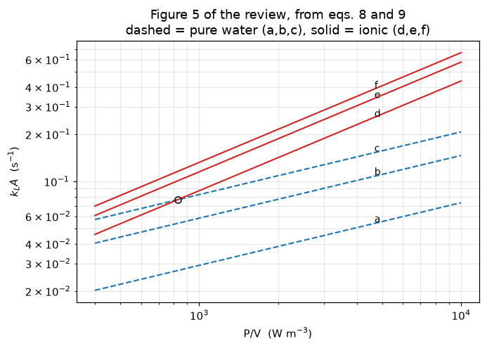
 pair    PV_cross  in_window
a x d     25.8294      False
a x e     10.2504      False
a x f      6.4574      False
b x d    260.3442      False
b x e    103.3176      False
b x f     65.0860      False
c x d    826.5412       True
c x e    328.0131      False
c x f    206.6353      False

crossings inside the plotted window 4e2..1e4: 1 (pair c x d, at P/V = 826.5 W/m3); nearest crossing to an edge 0.20 in ln(P/V)
window left edge 400 W/m3 = Figure 5's printed axis label 4.10^2 (transcribed text, not a measured coordinate)
the count is 1 for any left edge in (328.0, 826.5] W/m3; at the printed validity bound 500 it is 1; at 300 it would be 2
Exactly one of the nine candidate crossings falls inside the plotted window (the count and its position are printed above): the pure-water curve at 4 cm s⁻¹ (c) meeting the ionic curve at 0.5 cm s⁻¹ (d), a little to the left of the 10³ gridline. The review’s printed Figure 5 shows exactly one crossing, between exactly that pair, in exactly that position.
That is a real check on the transcription of both branches at once, and it is a sharp one: it reads all six constants. It is stated qualitatively on purpose. The abscissa of the printed crossing is not measured, because measuring it would be figure digitisation and this page does none. What is compared is the count and the identity of the pair, both of which are legible without extracting a coordinate.
Where the window comes from, and how much hangs on it. The window’s edges are Figure 5’s printed axis labels, 4.10² and 10⁴ on the abscissa: transcription of typeset text, not a measured coordinate, declared here because the left edge is load-bearing. The cell prints the interval of left edges for which the count is one, and the count at the printed validity bound, which is also one.
2. Which of the six constants the data actually exercise
The review poses this question about itself and does not answer it:
“Relatively much store is set by the values of \(\alpha\) and \(\beta\). To what extent these can be varied without affecting the outcome significantly will be discussed in more detail in the section on \(k_\mathrm{L}A\).”
It never is. The answer is computable from printed numbers alone, and the method matters: changing an exponent alone is not the comparison to make, because a reader who preferred a different exponent would re-fit the prefactor with it. The review says as much: “it correlates a great deal with \(\alpha\) because \(P/V = 10^3\!-\!10^4\)”. So re-fit \(K\) so the altered correlation is exact at the geometric centre of the printed window, and ask how far it can then stray anywhere inside that window. Compare against the review’s own claimed accuracy, 20 to 40 %.
rows = []
def add(branch, sym, alt, ref, lo, hi, what):
    cost, fac = refit_cost(alt, ref, lo, hi, what)
    rows.append(dict(branch=branch, exponent=sym, printed=ref, alternative=alt,
                     lo_end=fac[0], hi_end=fac[1], worst_dev=cost,
                     inside_accuracy=cost <= P0["acc_hi"]))

for a in (P0["alpha_purewater_lo"], P0["alpha_purewater_hi"], 0.0):
    add("pure_water", "alpha", a, CORR["pure_water"]["alpha"], *P0["pv_win"], "pv")
for b in (P0["beta_purewater_lo"], P0["beta_purewater_hi"], 0.0):
    add("pure_water", "beta", b, CORR["pure_water"]["beta"], *P0["vs_pure"], "vs")
for a in (0.4, 1.0, 0.0):                 # the general literature range of alpha, and zero
    add("ionic", "alpha", a, CORR["ionic"]["alpha"], *P0["pv_win"], "pv")
for b in (0.0, 0.7):                      # the general literature range of beta
    add("ionic", "beta", b, CORR["ionic"]["beta"], *P0["vs_ion"], "vs")
tol = pd.DataFrame(rows)
print(tol.to_string(index=False, float_format=lambda v: f"{v:8.4f}"))

print("\nNULL BASELINE: what each term buys over dropping it entirely")
print("  (prefactor re-fitted at the window centre in every case)")
for (br, sym), key in [(("pure_water", "alpha"), "null_pure_alpha0_cost"),
                       (("pure_water", "beta"), "null_pure_beta0_cost"),
                       (("ionic", "alpha"), "null_ion_alpha0_cost"),
                       (("ionic", "beta"), "null_ion_beta0_cost")]:
    c = A[key]
    verdict = "inside the review's own 20-40 % band" if c <= P0["acc_hi"] else "outside it"
    print(f"  {br:11s} {sym:5s} -> 0 : worst {100*c:6.1f} %   {verdict}")
# The ionic span: Figure 4's two DRAWN LINES (C1, C2) and the wider span its
# DATA occupy (Hassan 1977 to Reith 1968), both straight from the legend rows.
print(f"\nionic beta -> 0 over two spans: {100*A['null_ion_beta0_cost']:.1f} % over the drawn "
      f"lines C1..C2 ({P0['vs_ion'][0]}-{P0['vs_ion'][1]} m/s); "
      f"{100*A['null_ion_beta0_cost_dataspan']:.1f} % over the data span "
      f"({P0['vs_ion_data'][0]}-{P0['vs_ion_data'][1]} m/s); the review's accuracy "
      f"ceiling is {100*P0['acc_hi']:.0f} %")
print(f"pure-water literature spread: alpha {P0['alpha_purewater_lo']}-{P0['alpha_purewater_hi']} "
      f"costs at most {100*A['purewater_alpha_range_cost']:.1f} %, beta "
      f"{P0['beta_purewater_lo']}-{P0['beta_purewater_hi']} at most "
      f"{100*A['purewater_beta_range_cost']:.1f} %")
print(f"\nNULL BASELINE: dropping the BRANCHING and using eq. 8 for ionic systems "
      f"under-predicts by up to {100*A['null_single_branch_worst']:.1f} % "
      f"(ratio up to {A['ion_ratio_max']:.2f}x)")
branch exponent printed alternative lo_end hi_end worst_dev inside_accuracy
pure_water alpha 0.4000 0.3500 1.0778 0.9278 0.0778 True
pure_water alpha 0.4000 0.5000 0.8609 1.1616 0.1616 True
pure_water alpha 0.4000 0.0000 1.8206 0.5493 0.8206 False
pure_water beta 0.5000 0.3000 1.2470 0.8019 0.2470 True
pure_water beta 0.5000 0.6000 0.8955 1.1167 0.1167 True
pure_water beta 0.5000 0.0000 1.7364 0.5759 0.7364 False
ionic alpha 0.7000 0.4000 1.5673 0.6380 0.5673 False
ionic alpha 0.7000 1.0000 0.6380 1.5673 0.5673 False
ionic alpha 0.7000 0.0000 2.8534 0.3505 1.8534 False
ionic beta 0.2000 0.0000 1.2644 0.7909 0.2644 True
ionic beta 0.2000 0.7000 0.5563 1.7977 0.7977 False
NULL BASELINE: what each term buys over dropping it entirely
(prefactor re-fitted at the window centre in every case)
pure_water alpha -> 0 : worst 82.1 % outside it
pure_water beta -> 0 : worst 73.6 % outside it
ionic alpha -> 0 : worst 185.3 % outside it
ionic beta -> 0 : worst 26.4 % inside the review's own 20-40 % band
ionic beta -> 0 over two spans: 26.4 % over the drawn lines C1..C2 (0.0045-0.047 m/s); 35.2 % over the data span (0.0023-0.047 m/s); the review's accuracy ceiling is 40 %
pure-water literature spread: alpha 0.35-0.5 costs at most 16.2 %, beta 0.3-0.6 at most 24.7 %
NULL BASELINE: dropping the BRANCHING and using eq. 8 for ionic systems under-predicts by up to 83.3 % (ratio up to 5.98x)The four exponents are not equally earned.
Three of them are load-bearing. Dropping the \(P/V\) term on either branch, or the pure-water \(v_\mathrm{s}\) term, costs more than the 20 to 40 % the review claims for its own formulas (the cell prints each cost), so the data must be resolving them.
The fourth is not. Deleting the ionic \(v_\mathrm{s}\) term outright, setting \(\beta = 0\) and re-fitting the prefactor, changes the prediction by less than the review’s own accuracy both across the span of Figure 4’s two drawn correlation lines and across the wider span the figure’s data occupy (Hassan to Reith); the second sits near the top of the band. The exponent 0.2 on the ionic branch is not resolved by the review’s own error bar.
That is not a criticism the review would resist; it is what the review itself reports its sources as finding, and this page only puts the number on it:
“Westerterp et al. (1963) and also Reith and Beek (1968) claim that at \(v_\mathrm{s} > 0.5\) the superficial gas velocity exerts only a slight influence. Zlokarnik (1970) has found a slightly better correlation with \(v_\mathrm{s}^{0.2}\) than with \(v_\mathrm{s}^{0}\).”
The 0.2 was imported from Zlokarnik, not fitted on Figure 4: the review says so in the sentence that introduces eq. 9, and then \(K\) and \(\alpha\) were fitted with it held. So it is not surprising that it sits inside the noise; what is worth having is how far inside.
Within the pure-water literature spread the review quotes, \(\alpha\) = 0.35 to 0.5 and \(\beta\) = 0.3 to 0.6, the whole range stays inside the accuracy band once \(K\) is re-fitted. The spread in the literature exponents is not a disagreement about physics; it is what a 20 to 40 % correlation looks like.
3. The branching, against the review’s own expectation for it
The review expects ions to raise \(k_\mathrm{L}A\) by 2 to 10 times, and it builds that expectation mechanistically: interfacial area up to 10× (Lee & Meyrick), holdup up to 2× (Machón et al.), \(k_\mathrm{L}\) lower by at most 1 to 4×, then corroborated against Zlokarnik (1975). None of that comes from eqs. 8 and 9. So the ratio of the two fitted correlations is a genuine check against an independently-argued number, and it can fail.
\[\frac{\text{eq. 9}}{\text{eq. 8}} = \frac{2.0\times10^{-3}}{2.6\times10^{-2}} \left(\frac{P/V}{v_\mathrm{s}}\right)^{0.3}\]
The ratio is monotone in both variables, so its extremes are at two corners of the box (500 to 10 000 W m⁻³, and Figure 5’s velocities), fixed by the signs of the exponent differences; no grid search is involved. The share of the box where it lies between 2 and 10 is the area, in logarithmic coordinates, of the box clipped by two straight lines (log_box_fraction); it is what a uniform geometric grid converges to.
lo, hi = P0["ion_enhancement_lo"], P0["ion_enhancement_hi"]
PVG, VSG = np.geomspace(*P0["pv_win"], 200), np.geomspace(VS_FIG5[0], VS_FIG5[-1], 200)  # plotting grid
Rg = kla(PVG[:, None], VSG[None, :], "ionic") / kla(PVG[:, None], VSG[None, :], "pure_water")
fig, ax = plt.subplots(figsize=(6.0, 4.2))
cs = ax.contourf(PVG, VSG, Rg.T, levels=np.linspace(1, 7, 25), cmap="viridis")
ax.contour(PVG, VSG, Rg.T, levels=[lo], colors="w", linewidths=2)
ax.set_xscale("log"); ax.set_yscale("log")
ax.set_xlabel("P/V  (W m$^{-3}$)"); ax.set_ylabel("$v_s$  (m s$^{-1}$)")
ax.set_title(f"eq. 9 / eq. 8 over the printed window\nwhite line = the review's lower "
             f"expectation, {lo:g}x")
plt.colorbar(cs, ax=ax, label="enhancement factor"); plt.tight_layout(); plt.show()

print(f"d ln R/d ln(P/V) = {A['_da']:+.1f}, d ln R/d ln(v_s) = {A['_db']:+.1f}: the minimum is at "
      f"P/V = {A['_corner_min'][0]:.0f} W/m3, v_s = {A['_corner_min'][1]:.3f} m/s")
print(f"ratio spans {A['ion_ratio_min']:.4f} to {A['ion_ratio_max']:.4f} over the box")
print(f"the review expects {lo:g}-{hi:g}x; the two correlations deliver that on "
      f"{100*A['ion_ratio_frac_in_2_10']:.1f} % of the box (log-area share)")
print(f"the minimum falls {100*A['_floor_margin']:.1f} % short of the {lo:g}x floor")
print()
print("the review's two qualitative claims about the branching, as signs:")
print(f"  'increases at higher P/V values'        : {A['_da']:+.1f} > 0 "
      f"-> {'holds' if A['ratio_rises_with_pv'] else 'FAILS'}")
print(f"  'more dependent on P/V than pure water' : alpha {CORR['ionic']['alpha']} vs "
      f"{CORR['pure_water']['alpha']} -> {'holds' if A['ratio_rises_with_pv'] else 'FAILS'}")
print(f"  (and the enhancement FALLS with v_s     : {A['_db']:+.1f} < 0, "
      f"which the review does not state)")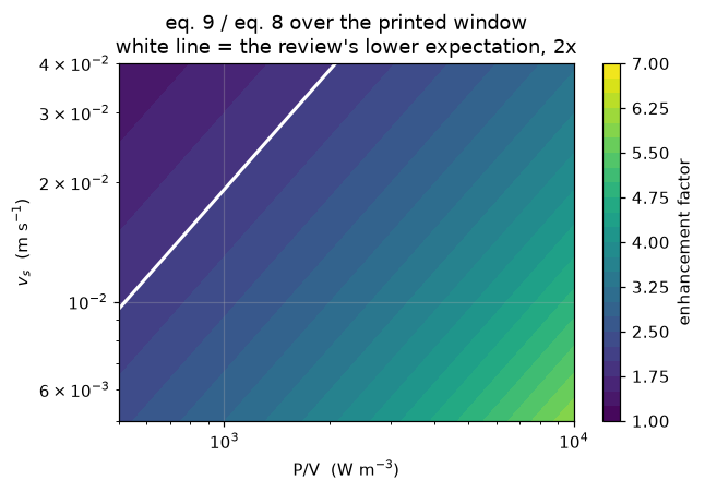
d ln R/d ln(P/V) = +0.3, d ln R/d ln(v_s) = -0.3: the minimum is at P/V = 500 W/m3, v_s = 0.040 m/s
ratio spans 1.3036 to 5.9754 over the box
the review expects 2-10x; the two correlations deliver that on 83.7 % of the box (log-area share)
the minimum falls 34.8 % short of the 2x floor

the review's two qualitative claims about the branching, as signs:
  'increases at higher P/V values'        : +0.3 > 0 -> holds
  'more dependent on P/V than pure water' : alpha 0.7 vs 0.4 -> holds
  (and the enhancement FALLS with v_s     : -0.3 < 0, which the review does not state)
The review’s qualitative claims about the branching are recovered exactly: the enhancement does grow with \(P/V\), because \(0.7 > 0.4\), which is the sentence “the \(k_\mathrm{L}A\)’s for ionic solutions are more dependent on \(P/V\) than those for pure water”. The two correlations land inside the review’s expected 2 to 10× on the share of the box the cell prints.
But the corner at high \(v_\mathrm{s}\) and low \(P/V\) falls below the 2× floor the review argues for. The two things are printed four pages apart, and neither is derived from the other, so this is a genuine internal inconsistency rather than an arithmetic slip: at 4 cm s⁻¹ and 500 W m⁻³ the review’s own fitted correlations say adding salt barely changes \(k_\mathrm{L}A\), while its own mechanistic argument says it must at least double it. The page reports it and does not resolve it; the evidence that would settle it is in Figures 3 and 4, which are not digitised.
The branch null baseline (Results 2) is the other half of this: using eq. 8 for an ionic system under-predicts by up to the share printed there. The branching is the single most load-bearing feature of the correlation, which is why a page that checked only one branch would be worthless.
4. Where the correlation outgrows the method that produced it
The review states, precisely, how fast a \(k_\mathrm{L}A\) a normal electrode can follow: “commercially available electrodes with \(\tau_\mathrm{p}\) = 2 or 3 s to \(k_\mathrm{L}A = 0.1\) s⁻¹”. That ceiling is not a free-standing number: it is Linek’s criterion \(\tau_\mathrm{p} \le 1/(5k_\mathrm{L}A)\) evaluated at \(\tau_\mathrm{p}\) = 2 s, and recovering it is a check on three separate transcriptions at once. The share of the window above the ceiling is again a log-area share in closed form, over \(P/V\) = 500 to 10 000 W m⁻³ and Figure 4’s C1..C2 span of \(v_\mathrm{s}\).
ceil = P0["kla_electrode_ceiling"]
print("recovering the printed electrode ceiling from the printed probe criteria")
for t in (P0["probe_tau_lo"], P0["probe_tau_hi"]):
    print(f"  tau_p = {t:.0f} s :  Linek       (<3% err) k_LA <= 1/(5 tau_p) = "
          f"{1/(P0['linek_margin']*t):.4f} 1/s")
    print(f"              :  Van de Sande (<6% err) k_LA <= 1/tau_p        = {1/t:.4f} 1/s")
print(f"  printed ceiling = {ceil} 1/s; 1/(5 x {P0['probe_tau_lo']:.0f} s) = "
      f"{A['electrode_ceiling_from_linek']:.4f} 1/s (relative gap {A['ceiling_closure_gap']:.1e})")

PVW, VSW = np.geomspace(*P0["pv_win"], 200), np.geomspace(*P0["vs_ion"], 200)    # plotting grid
fig, ax = plt.subplots(figsize=(6.0, 4.2))
for (br, tag), col in zip(BRANCHES, ("C0", "C3")):
    ax.contour(PVW, VSW, kla(PVW[:, None], VSW[None, :], br).T, levels=[ceil], colors=col, linewidths=2)
    print(f"  {br:11s}: {100*A[f'frac_window_above_ceiling_{tag}']:5.1f} % of the window (log-area share) lies above "
          f"k_LA = {ceil} 1/s")
ax.set_xscale("log"); ax.set_yscale("log")
ax.set_xlabel("P/V  (W m$^{-3}$)"); ax.set_ylabel("$v_s$  (m s$^{-1}$)")
ax.set_title(f"where each branch reaches $k_LA$ = {ceil} s$^{{-1}}$\n"
             "blue = eq. 8 (pure water), red = eq. 9 (ionic)")
ax.grid(True, which="both", alpha=.3); plt.tight_layout(); plt.show()
for v in VS_FIG5:
    p8 = (ceil / (CORR["pure_water"]["K"] * v**CORR["pure_water"]["beta"]))**(1/CORR["pure_water"]["alpha"])
    p9 = (ceil / (CORR["ionic"]["K"] * v**CORR["ionic"]["beta"]))**(1/CORR["ionic"]["alpha"])
    print(f"  v_s = {v:.3f} m/s : reached at P/V = {p8:8.0f} (pure) and {p9:8.0f} (ionic) W/m3")
print(f"\n  the ionic branch is above the ceiling everywhere past P/V = "
      f"{A['pv_where_ionic_passes_ceiling']:.0f} W/m3, at every v_s Figure 5 draws")
recovering the printed electrode ceiling from the printed probe criteria
tau_p = 2 s : Linek (<3% err) k_LA <= 1/(5 tau_p) = 0.1000 1/s
: Van de Sande (<6% err) k_LA <= 1/tau_p = 0.5000 1/s
tau_p = 3 s : Linek (<3% err) k_LA <= 1/(5 tau_p) = 0.0667 1/s
: Van de Sande (<6% err) k_LA <= 1/tau_p = 0.3333 1/s
printed ceiling = 0.1 1/s; 1/(5 x 2 s) = 0.1000 1/s (relative gap 0.0e+00)
pure_water : 23.2 % of the window (log-area share) lies above k_LA = 0.1 1/s
ionic : 80.5 % of the window (log-area share) lies above k_LA = 0.1 1/s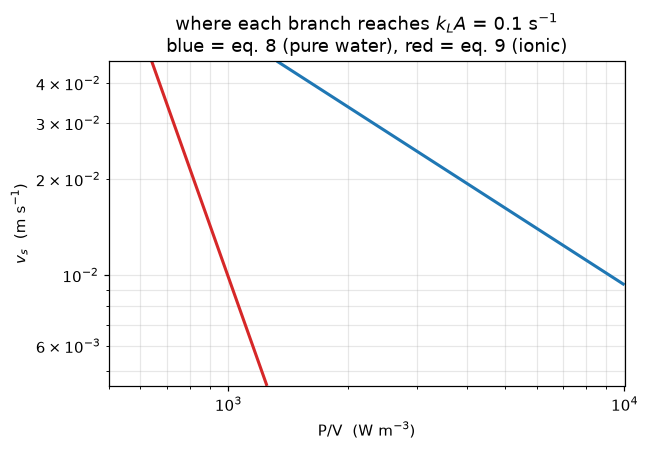
  v_s = 0.005 m/s : reached at P/V =    21820 (pure) and     1215 (ionic) W/m3
  v_s = 0.020 m/s : reached at P/V =     3857 (pure) and      818 (ionic) W/m3
  v_s = 0.040 m/s : reached at P/V =     1622 (pure) and      671 (ionic) W/m3

  the ionic branch is above the ceiling everywhere past P/V = 1215 W/m3, at every v_s Figure 5 draws
\(1/(5\times 2\,\mathrm{s}) = 0.1\) s⁻¹: the review’s printed ceiling is exactly Linek’s tighter criterion at the faster of the two electrodes it names. Three numbers read off a scan, and they close.
Applied to the correlations, the two branches behave completely differently (the shares are printed above). Eq. 8 stays below the ceiling over most of the window, while eq. 9 is above it over most of it, and has crossed it by the printed \(P/V\) at every velocity Figure 5 draws. So most of the ionic correlation’s own validity window lies in the regime where the review says a response model is required. That is not a contradiction: the review says plainly that with response models “one can measure up to values several times higher”. But it does say that the ionic branch is, over most of its range, a correlation of corrected measurements rather than raw ones, and the review’s own warning about how much accuracy those corrections cost applies to it far more than to eq. 8.
5. What the well-mixed-gas assumption costs: the pymrm part
Everything above is arithmetic on printed constants. This is the part that needs a model.
Eq. 2 assumes the gas composition is uniform and equal to the inlet. The review returns to that four times, gives the residence time that governs it (eq. 3), says the problem worsens with vessel size and at low \(v_\mathrm{s}\), and stops. With the plug-flow column solved, the cost becomes a number: \(\varphi\), the ratio of the true column-mean driving force to the one eq. 2 assumes. The \(k_\mathrm{L}A\) an experimenter reports is \(\varphi\) times the real one in the quasi-steady limit; the full transient (Validation) gives what eq. 2 actually returns.
print(f"worked vessel: V = {W0['V']*1e3:.0f} L, T/H = {W0['th']}, so H_t = {H_T:.4f} m and "
      f"T = {W0['th']*H_T:.4f} m (from the review's own eq. 3 geometry)")
print(f"worked point : P/V = {PV0:.1f} W/m3 (geometric centre of the printed window), "
      f"v_s = {VS0} m/s (the lowest velocity Figure 5 draws)\n")
dep = pd.DataFrame([dict(branch=br, kLA=A[f"kLA_{tag}_worked"], N_G=A[f"NG_times_H_{tag}"] / HENRY,
                         N_G_times_H=A[f"NG_times_H_{tag}"],
                         tauG_times_kLA=A["tau_G_worked"] * A[f"kLA_{tag}_worked"],
                         phi=A[f"phi_{tag}"], bias_pct=100 * A[f"bias_{tag}_quasisteady"],
                         one_over_k_phi=A[f"liquid_time_{tag}"]) for br, tag in BRANCHES])
print(dep.to_string(index=False, float_format=lambda v: f"{v:9.4f}"))
print(f"\ntau_G = {A['tau_G_worked']:.1f} s; eq. 9 predicts {A['k_ratio_worked']:.1f}x eq. 8's "
      "transfer coefficient here, hence the same factor on N_G")
print("`tauG_times_kLA` is the review's OWN criterion; `N_G` is the one the balance gives.")
print(f"they differ by the factor (1-eps)/(eps H) = {A['criterion_factor']:.4f}, "
      "which the review's criterion omits.")
print(f"V as dispersion volume: at eps = {EPS} the dispersion height is larger by (1-eps)^(-1/3), "
      f"+{100*A['dispersion_height_NG_effect']:.1f} % on N_G")
worked vessel: V = 2600 L, T/H = 1.0, so H_t = 1.4904 m and T = 1.4904 m (from the review's own eq. 3 geometry)
worked point : P/V = 2236.1 W/m3 (geometric centre of the printed window), v_s = 0.005 m/s (the lowest velocity Figure 5 draws)
branch kLA N_G N_G_times_H tauG_times_kLA phi bias_pct one_over_k_phi
pure_water 0.0402 0.3595 10.7850 1.1983 0.8400 16.0014 29.6125
ionic 0.1533 1.3706 41.1179 4.5687 0.5443 45.5679 11.9862
tau_G = 29.8 s; eq. 9 predicts 3.8x eq. 8's transfer coefficient here, hence the same factor on N_G
`tauG_times_kLA` is the review's OWN criterion; `N_G` is the one the balance gives.
they differ by the factor (1-eps)/(eps H) = 0.3000, which the review's criterion omits.
V as dispersion volume: at eps = 0.1 the dispersion height is larger by (1-eps)^(-1/3), +3.6 % on N_G# the vessel-size dependence the review asserts and never quantifies,
# run over the vessel volumes its own figure legends print (T/H held at the centre)
size = pd.DataFrame([dict(V_L=V, H_t=height(V * 1e-3, W0["th"]),
**{f"bias_{br}_pct": 100 * (1 - float(phi_closed(stripping_number(
float(kla(PV0, VS0, br)), height(V * 1e-3, W0["th"]), VS0, EPS, HENRY))))
for br, _ in BRANCHES})
for V in V_PRINTED])
print(f"at P/V = {PV0:.0f} W/m3 and v_s = {VS0} m/s, over the printed vessel volumes:\n")
print(size.to_string(index=False, float_format=lambda v: f"{v:9.4f}"))
print(f"\nionic quasi-steady bias: {100*A['bias_ionic_2p5L']:.1f} % at {P0['v_printed'][0]:g} L, "
f"{100*A['bias_ionic_5100L']:.1f} % at {P0['v_printed'][1]:g} L")
fig, ax = plt.subplots(figsize=(6.0, 4.0))
for (br, _), col, lab in zip(BRANCHES, ("C0", "C3"), ("eq. 8, pure water", "eq. 9, ionic")):
ax.semilogx(size.V_L, size[f"bias_{br}_pct"], "o-", color=col, label=lab)
ax.set_xlabel("vessel volume (L), from the figure legends")
ax.set_ylabel("bias in $k_LA$ from eq. 2 (%)")
ax.set_title("how much the well-mixed-gas assumption under-reports $k_LA$ (quasi-steady)")
ax.legend(); ax.grid(alpha=.3); plt.tight_layout(); plt.show()at P/V = 2236 W/m3 and v_s = 0.005 m/s, over the printed vessel volumes:
V_L H_t bias_pure_water_pct bias_ionic_pct
2.5000 0.1471 1.7534 6.4690
5.0000 0.1853 2.2023 8.0578
21.0000 0.2990 3.5213 12.5715
40.0000 0.3707 4.3403 15.2618
70.0000 0.4467 5.1990 17.9936
90.0000 0.4857 5.6359 19.3492
180.0000 0.6120 7.0306 23.5268
1360.0000 1.2008 13.1802 39.4594
4400.0000 1.7760 18.6630 50.7309
5100.0000 1.8656 19.4736 52.1967
ionic quasi-steady bias: 6.5 % at 2.5 L, 52.2 % at 5100 L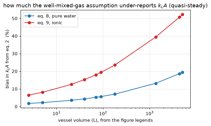
The two cells above give, at the geometric centre of the printed \(P/V\) window, at the lowest velocity Figure 5 draws, in the largest vessel eq. 8 claims, the transfer coefficient, \(N_\mathrm{G}\), \(\varphi\) and the quasi-steady under-report of each branch.
The \(\varphi\)’s are quasi-steady, and the page’s own transient says the quasi-steady number is the optimistic one on the pure-water branch. \(\varphi = (1-e^{-N_G})/N_G\) freezes the gas column, which is valid when \(\tau_\mathrm{G} \ll 1/k_\mathrm{L}A\): exactly the condition being shown to fail (\(\tau_\mathrm{G}\) and \(1/(k\varphi)\) are printed above, and they are of the same order). Solving the full transient gassing-out experiment and applying eq. 2 to the trace (Validation) gives a larger under-report on the pure-water branch. On the ionic branch the two timescales are farthest apart, the response is not a single exponential, and what eq. 2 returns therefore depends on where the trace is fitted; Validation prints the sweep over three fit windows, with the quasi-steady value inside its range. The transient numbers lead the headline; \(\varphi\) is kept beside them because it is closed-form, deterministic and free of any window choice.
The branch matters more here than anywhere else on the page. The whole difference between the branches comes from the four constants: eq. 9 predicts several times the transfer coefficient at this point (printed above), hence the same factor on the stripping number in the same gas stream. The ionic bias is of the same size as the entire accuracy the review claims for its formulas.
And across the vessel sizes the review’s own legends print, the effect grows from the bench vessel to Calderbank’s 5100 L one, which is precisely the review’s sentence “Problems become more serious at larger vessel diameter especially at low superficial gas velocity values”, with numbers on it. The direction, the vessel-size trend and the \(v_\mathrm{s}\) trend are all the review’s own claims; what is new is the magnitude, and the fact that it is branch-dependent.
Three qualifications, all load-bearing.
This is a statement about the correlation’s self-consistency, not a correction to it. If the underlying measurements were biased low by \(\varphi\), then eq. 9 as fitted already contains that bias, and dividing by \(\varphi\) would double-count. What the calculation establishes is that eq. 9, taken at face value, predicts conditions under which the method that produced most of its data does not measure what it is assumed to measure.
\(H\) is not printed in the review. \(N_\mathrm{G}\) is inversely proportional to it, so the numbers above move with it; Validation sweeps \(H\) = 20 to 40 and reports the range, and the \(H\)-free group \(N_\mathrm{G}H\) is printed beside them.
\(V\) does double duty as liquid volume and dispersion volume. The review’s Nomenclature defines \(V\) as the fluid volume; this page sets \(H_\mathrm{t}\) from \(V = \tfrac14\pi T^2 H_\mathrm{t}\) and then uses that \(H_\mathrm{t}\) as the dispersion height in \(N_\mathrm{G}\). With the aspect ratio held, the dispersion height is larger by \((1-\epsilon)^{-1/3}\), the effect on \(N_\mathrm{G}\) printed above: inside the \(\epsilon\)-sweep envelope, and the same identification the review’s own eq. 3 makes.
Validation
This page is a REPRODUCTION, NOT A VALIDATION, and the distinction is not cosmetic here. Eqs. 8 and 9 were fitted by van ’t Riet to the literature data he compiles in Figures 1 to 5. Any agreement between them and those data would be a goodness of fit, not a test, and this page cannot even compute that, because the data live only in the figures and figure extraction needs a maintainer review that is not available. The data tier is 6. No measurement is compared against anywhere on this page.
What can be checked, and is:
- the pymrm column against a closed form derived independently of it, on a cell ladder;
- the pymrm transient on separate ladders in the time step and in the cells, and against a Lagrangian route that forms no spatial operator, on its own ladder;
- a global oxygen balance across the two phases, read at the faces;
- the review’s internal identities: eq. 3’s two forms, and the electrode ceiling recovered from the two probe criteria;
- a defect-injection table in which every claim has a row that fails it.
Every order comes from successive differences of at least three levels (pymrm.checks.observed_orders), never against the finest level, with a companion claim that the finest differences are far above the solves’ round-off.
NS_COL = (100, 200, 400, 800, 1600)


def orders(f, ns, ratio=None):
    """observed_orders on the ladder ``ns``; ``ratio`` reads it with another ratio (a defect)."""
    if ratio is None:
        return observed_orders(f, ns)
    lab = {int(round(64 * ratio**i)): n for i, n in enumerate(ns)}
    return observed_orders(lambda m: f(lab[m]), tuple(lab))


def column_study(ns=NS_COL, read="face", ratio=None, **kw):
    """The quasi-steady column against phi_closed on a cell ladder, both branches."""
    out = {}
    for br, tag in BRANCHES:
        k = float(kla(PV0, VS0, br))
        exact = float(phi_closed(stripping_number(k, H_T, VS0, EPS, HENRY)))
        runs = {n: phi_pymrm(n, H_T, VS0, EPS, k, HENRY, C_in=C_IN, return_balance=True, read=read, **kw)
                for n in ns}
        oo = orders(lambda n: runs[n][0], ns, ratio)
        out[f"pymrm_vs_closed_n1600_{tag}"] = abs(runs[ns[-1]][0] / exact - 1)
        out[f"pymrm_vs_closed_richardson_{tag}"] = abs(oo["extrapolated"] / exact - 1)
        out[f"grid_order_{tag}_min"] = float(np.min(oo["orders"]))
        out[f"grid_order_{tag}_max"] = float(np.max(oo["orders"]))
        out[f"_finest_{tag}"] = abs(runs[ns[-1]][0] - runs[ns[-2]][0])
        out[f"_gap_{tag}"] = max(r[1] for r in runs.values())
        out[f"_runs_{tag}"], out[f"_exact_{tag}"] = runs, exact
    return out


COL = column_study()
print("=== 1. pymrm column against the closed form (1 - exp(-N_G))/N_G, cell ladder ===")
for br, tag in BRANCHES:
    runs = COL[f"_runs_{tag}"]
    print(f"  {br:11s} n = {NS_COL}: rel err "
          f"{', '.join(f'{abs(runs[n][0] / COL[f'_exact_{tag}'] - 1):.3e}' for n in NS_COL)}")
    print(f"  {'':11s} orders {COL[f'grid_order_{tag}_min']:.4f} to {COL[f'grid_order_{tag}_max']:.4f} "
          f"(first-order upwind: 1); Richardson limit against the closed form "
          f"{COL[f'pymrm_vs_closed_richardson_{tag}']:.1e}")
    print(f"  {'':11s} column balance (face fluxes against summed transfer) below 1e-12 "
          f"(here {COL[f'_gap_{tag}']:.1e})")
=== 1. pymrm column against the closed form (1 - exp(-N_G))/N_G, cell ladder ===
pure_water n = (100, 200, 400, 800, 1600): rel err 1.491e-03, 7.461e-04, 3.732e-04, 1.867e-04, 9.335e-05
orders 0.9978 to 0.9994 (first-order upwind: 1); Richardson limit against the closed form 4.8e-08
column balance (face fluxes against summed transfer) below 1e-12 (here 5.3e-13)
ionic n = (100, 200, 400, 800, 1600): rel err 3.183e-03, 1.595e-03, 7.984e-04, 3.994e-04, 1.998e-04
orders 0.9952 to 0.9988 (first-order upwind: 1); Richardson limit against the closed form 2.2e-07
column balance (face fluxes against summed transfer) below 1e-12 (here 5.0e-14)The transient. The time ladder refines the step at 800 cells and the cell ladder refines the cells at 4000 steps; successive differences cancel the other axis’s fixed error, so each ladder gives its own order. Each limit is the first-order Richardson value of its ladder; the two corrections added to the production run (800 cells, 4000 steps) give the two-axis limit. The crossing times are roots of the piecewise-linear interpolant of the trace (crossing_time, find_roots on the whole trace, exactly one root or it raises); the interpolation error is second order in the step and sits inside the time ladder. The Lagrangian route refines its age step and output step together.
On the ionic branch the (0.2, 0.8) window closes before the first gas parcel that entered after \(t = 0\) reaches the outlet (\(t_2 < \tau_\mathrm{G}\)). Until then the outlet face carries gas that was in the column at \(t = 0\), whose state is the same in every cell, and with a linear sink the column mean obeys a closed balance: the trace does not depend on the cells, to round-off. The cell ladder shows it, and the claim records the margin of \(t_2\) to \(\tau_\mathrm{G}\).
NT_LAD, N_LAD = (500, 1000, 2000, 4000), (200, 400, 800, 1600)
N_PROD, NT_PROD = 800, 4000
LAG_LAD = ((200, 2000), (400, 4000), (800, 8000), (1600, 16000))
WINDOWS = ((0.2, 0.8), (0.1, 0.9), (0.3, 0.7))


def transient_study(br, nts=NT_LAD, ns=N_LAD, lag=LAG_LAD, window=(0.2, 0.8), read="face",
                    t_ratio=None, s_ratio=None, l_ratio=None, **kw):
    """Gassing out on a time ladder and a cell ladder, eq. 2 applied, and the Lagrangian route.

    The ``*_ratio`` arguments override the refinement ratio the ladders are read
    with (a defect-injection switch); the limits use first-order Richardson.
    """
    tag = dict(BRANCHES)[br]
    k = float(kla(PV0, VS0, br))
    phi = float(phi_closed(stripping_number(k, H_T, VS0, EPS, HENRY)))
    t_end, C_star = 6.0 / (k * phi), C_IN / HENRY
    wins = (window,) + WINDOWS[1:]
    runs = {}

    def q(n, nt, inert):
        if (n, nt, inert) not in runs:
            ts, CL, _, bal = gassing_out(n, nt, t_end, H_T, VS0, EPS, k, HENRY, C_in=C_IN,
                                         gas_initially_inert=inert, read=read, **kw)
            runs[(n, nt, inert)] = (np.array([fit_eq2(ts, CL, C_star, *w) / k for w in wins]), bal,
                                    crossing_time(ts, CL, wins[0][1] * C_star))
        return runs[(n, nt, inert)]

    n0, nt0 = ns[-2], nts[-1]
    rt, rs = t_ratio or nts[1] / nts[0], s_ratio or ns[1] / ns[0]
    out, lim, prod = {}, {}, {}
    t_ord, s_ord, finest = [], [], []
    for inert in (False, True):
        for j in range(len(wins)):
            tl = orders(lambda nt: q(n0, nt, inert)[0][j], nts, t_ratio)
            sl = orders(lambda n: q(n, nt0, inert)[0][j], ns, s_ratio)
            p = tl["values"][-1]                      # production: ns[-2] cells, nts[-1] steps
            # first-order Richardson corrections to the production run: the step is the
            # finest of its ladder, the cells are one below the finest of theirs
            t_corr = (tl["values"][-1] - tl["values"][-2]) / (rt - 1)
            s_corr = (sl["values"][-1] - sl["values"][-2]) * rs / (rs - 1)
            prod[(inert, j)], lim[(inert, j)] = p, p + t_corr + s_corr
            if j == 0:
                t_ord += list(tl["orders"]); s_ord += list(sl["orders"])
                finest += [abs(t_corr)] + ([abs(s_corr)] if br == "pure_water" else [])
                if not inert:
                    out[f"kapp_over_k_{tag}_richardson"] = p + t_corr
                    out["_s_effect"] = abs(s_corr)
    rl = l_ratio or lag[1][0] / lag[0][0]
    L = orders(lambda mn: fit_eq2(*lagrangian(*mn, t_end, H_T, VS0, EPS, k, HENRY, C_in=C_IN),
                                  C_star, *wins[0]) / k, list(lag), rl)    # (M, steps) refined together
    lag_lim = L["values"][-1] + (L["values"][-1] - L["values"][-2]) / (rl - 1)
    finest.append(abs(L["values"][-1] - L["values"][-2]))
    # every reported k_app/k is the two-axis limit; the production run is kept beside it
    out[f"kapp_over_k_{tag}"] = lim[(False, 0)]
    out[f"kapp_over_k_{tag}_production"] = prod[(False, 0)]
    out[f"bias_{tag}_transient"] = 1.0 - lim[(False, 0)]
    out[f"kapp_over_k_{tag}_inert_start"] = lim[(True, 0)]
    out[f"kapp_over_k_{tag}_w19"], out[f"kapp_over_k_{tag}_w37"] = lim[(False, 1)], lim[(False, 2)]
    out[f"kapp_disc_effect_{tag}"] = max(abs(lim[key] - prod[key]) for key in prod)
    out[f"time_order_{tag}_min"], out[f"time_order_{tag}_max"] = float(np.min(t_ord)), float(np.max(t_ord))
    out[f"o2_balance_{tag}"] = q(n0, nt0, False)[1]
    out[f"lagrangian_order_{tag}_min"] = float(np.min(L["orders"]))
    out[f"lagrangian_order_{tag}_max"] = float(np.max(L["orders"]))
    out[f"lagrangian_limit_gap_{tag}"] = abs(lag_lim / lim[(False, 0)] - 1)
    if br == "pure_water":
        out["space_order_pure_min"], out["space_order_pure_max"] = float(np.min(s_ord)), float(np.max(s_ord))
    else:
        out["kapp_space_effect_ionic"] = out.pop("_s_effect")
        tau_G = EPS * H_T / VS0
        t2 = q(n0, nt0, False)[2]
        out["ionic_fit_before_tau_G"] = bool(t2 < tau_G)
        out["_tau_margin"] = abs(1 - t2 / tau_G)
        out["kapp_over_k_ionic_inert_start_w19"] = lim[(True, 1)]
        out["kapp_over_k_ionic_inert_start_w37"] = lim[(True, 2)]
        w = [lim[(False, j)] for j in range(3)]
        out["bias_ionic_window_min"], out["bias_ionic_window_max"] = 1 - max(w), 1 - min(w)
        out["phi_ionic_inside_window_range"] = bool(min(w) < phi < max(w))
        out["_window_margin"] = min(abs(phi / x - 1) for x in w if x != w[0])
    out.pop("_s_effect", None)
    out["_finest"] = min(finest)
    out["_gap"] = max(r[1] for r in runs.values())
    out["_lag"], out["_lim"], out["_prod"], out["_phi"] = L, lim, prod, phi
    return out


TR = {br: transient_study(br) for br, _ in BRANCHES}
print("=== 2. the transient: eq. 2 applied to the gassing-out trace ===")
for br, tag in BRANCHES:
    s = TR[br]
    print(f"  {br:11s} k_app/k at {N_PROD} cells, {NT_PROD} steps = {s[f'kapp_over_k_{tag}_production']:.6f}; "
          f"step limit {s[f'kapp_over_k_{tag}_richardson']:.6f}; two-axis limit "
          f"{s[f'kapp_over_k_{tag}']:.6f}")
    print(f"  {'':11s} time orders {s[f'time_order_{tag}_min']:.4f} to {s[f'time_order_{tag}_max']:.4f} "
          f"(backward Euler: 1), steps {NT_LAD}")
    if br == "pure_water":
        print(f"  {'':11s} cell orders {s['space_order_pure_min']:.4f} to {s['space_order_pure_max']:.4f} "
              f"(upwind: 1), cells {N_LAD}")
    else:
        print(f"  {'':11s} cell effect on the (0.2, 0.8) fit below 1e-8 (here "
              f"{s['kapp_space_effect_ionic']:.1e}): t_2 is {100*s['_tau_margin']:.0f} % short of tau_G")
    print(f"  {'':11s} production run against the two-axis limit, any window or start: below 5e-3 "
          f"(here {s[f'kapp_disc_effect_{tag}']:.1e})")
    print(f"  {'':11s} phi (quasi-steady) = {s['_phi']:.6f}   (gas inventory neglected)")
    print(f"  {'':11s} Lagrangian route: orders {s[f'lagrangian_order_{tag}_min']:.4f} to "
          f"{s[f'lagrangian_order_{tag}_max']:.4f} on (M, steps) = {LAG_LAD}; its limit against the "
          f"two-axis limit below 1e-4 (here {s[f'lagrangian_limit_gap_{tag}']:.1e})")
    print(f"  {'':11s} gas inert at t = 0: k_app/k = {s[f'kapp_over_k_{tag}_inert_start']:.6f} "
          "(N2 still in the vessel at the switch; two-axis limit)")
    print(f"  {'':11s} O2 balance below 1e-8 (here {s[f'o2_balance_{tag}']:.1e}), faces read with "
          "compute_boundary_values")
    for j, (f1, f2) in enumerate(WINDOWS):
        print(f"  {'':11s} fit window ({f1:.1f}, {f2:.1f}): k_app/k = {s['_lim'][(False, j)]:.4f}"
              f"   inert start = {s['_lim'][(True, j)]:.4f}   (two-axis limits)")
si = TR["ionic"]
print(f"\nThe window matters on the ionic branch: tau_G = {A['tau_G_worked']:.1f} s exceeds the ionic "
      f"liquid time constant 1/(k phi) = {A['liquid_time_ionic']:.1f} s")
print(f"(pure water: 1/(k phi) = {A['liquid_time_pure']:.1f} s, comparable to tau_G), so the ionic "
      "response is two-timescale and not a single exponential.")
print(f"Eq. 2's ionic bias spans {100*si['bias_ionic_window_min']:.1f} to "
      f"{100*si['bias_ionic_window_max']:.1f} % over the three windows; the quasi-steady "
      f"{100*A['bias_ionic_quasisteady']:.1f} % lies inside that range, "
      f"{100*si['_window_margin']:.0f} % or more from either end window.")
print(f"Headline (two-axis limits): eq. 2 under-reports by {100*TR['pure_water']['bias_pure_transient']:.1f} % "
      f"(pure water; quasi-steady {100*A['bias_pure_quasisteady']:.1f} %) and "
      f"{100*si['bias_ionic_transient']:.1f} % (ionic, window (0.2, 0.8)).")
=== 2. the transient: eq. 2 applied to the gassing-out trace ===
pure_water k_app/k at 800 cells, 4000 steps = 0.808220; step limit 0.808738; two-axis limit 0.808914
time orders 0.9883 to 0.9934 (backward Euler: 1), steps (500, 1000, 2000, 4000)
cell orders 0.9943 to 0.9986 (upwind: 1), cells (200, 400, 800, 1600)
production run against the two-axis limit, any window or start: below 5e-3 (here 2.3e-03)
phi (quasi-steady) = 0.839986 (gas inventory neglected)
Lagrangian route: orders 1.0010 to 1.0198 on (M, steps) = ((200, 2000), (400, 4000), (800, 8000), (1600, 16000)); its limit against the two-axis limit below 1e-4 (here 1.2e-06)
gas inert at t = 0: k_app/k = 0.755626 (N2 still in the vessel at the switch; two-axis limit)
O2 balance below 1e-8 (here 1.4e-10), faces read with compute_boundary_values
fit window (0.2, 0.8): k_app/k = 0.8089 inert start = 0.7556 (two-axis limits)
fit window (0.1, 0.9): k_app/k = 0.8060 inert start = 0.7348 (two-axis limits)
fit window (0.3, 0.7): k_app/k = 0.8088 inert start = 0.7772 (two-axis limits)
ionic k_app/k at 800 cells, 4000 steps = 0.545917; step limit 0.546262; two-axis limit 0.546262
time orders 0.9890 to 0.9994 (backward Euler: 1), steps (500, 1000, 2000, 4000)
cell effect on the (0.2, 0.8) fit below 1e-8 (here 8.8e-13): t_2 is 39 % short of tau_G
production run against the two-axis limit, any window or start: below 5e-3 (here 8.1e-04)
phi (quasi-steady) = 0.544321 (gas inventory neglected)
Lagrangian route: orders 0.9928 to 0.9989 on (M, steps) = ((200, 2000), (400, 4000), (800, 8000), (1600, 16000)); its limit against the two-axis limit below 1e-4 (here 1.4e-06)
gas inert at t = 0: k_app/k = 0.284185 (N2 still in the vessel at the switch; two-axis limit)
O2 balance below 1e-8 (here 1.5e-10), faces read with compute_boundary_values
fit window (0.2, 0.8): k_app/k = 0.5463 inert start = 0.2842 (two-axis limits)
fit window (0.1, 0.9): k_app/k = 0.4350 inert start = 0.2804 (two-axis limits)
fit window (0.3, 0.7): k_app/k = 0.6594 inert start = 0.2915 (two-axis limits)
The window matters on the ionic branch: tau_G = 29.8 s exceeds the ionic liquid time constant 1/(k phi) = 12.0 s
(pure water: 1/(k phi) = 29.6 s, comparable to tau_G), so the ionic response is two-timescale and not a single exponential.
Eq. 2's ionic bias spans 34.1 to 56.5 % over the three windows; the quasi-steady 45.6 % lies inside that range, 17 % or more from either end window.
Headline (two-axis limits): eq. 2 under-reports by 19.1 % (pure water; quasi-steady 16.0 %) and 45.4 % (ionic, window (0.2, 0.8)).ROUNDOFF = max(COL["_gap_pure"], COL["_gap_ionic"], *(TR[b]["_gap"] for b, _ in BRANCHES))
FINEST = min(COL["_finest_pure"], COL["_finest_ionic"], *(TR[b]["_finest"] for b, _ in BRANCHES))
FINEST_OVER_ROUNDOFF = FINEST / ROUNDOFF
print("smallest finest difference of any ladder over the largest balance gap of the solves: "
f"at least 1e3 (here {FINEST_OVER_ROUNDOFF:.1e})")smallest finest difference of any ladder over the largest balance gap of the solves: at least 1e3 (here 4.8e+04)print("=== 3. the review's own identities ===")
print(f" eq. 3 two forms, eps V/(v_s pi T^2/4) and eps H_t/v_s: relative gap below 1e-12 "
f"(here {A['eq3_forms_gap']:.1e})")
print(" an identity of the cylinder once V = pi T^2 H_t/4; it confirms the geometry")
print(" convention (H_t is the dispersion height) and fails if the vessel is built wrong.")
print(f" electrode ceiling: 1/({P0['linek_margin']:.0f} x {P0['probe_tau_lo']:.0f} s) = "
f"{A['electrode_ceiling_from_linek']:.4f} 1/s vs printed {P0['kla_electrode_ceiling']:.4f} 1/s")
print(" three independently transcribed numbers close on the fourth.")
print("\n=== the unprinted inputs, swept ===")
for br, tag in BRANCHES:
print(f" {br:11s} N_G*H = {A[f'NG_times_H_{tag}']:.4f} (dimensionless, H-free) "
f"H=20: phi={A[f'phi_{tag}_H20']:.4f} H=30: phi={A[f'phi_{tag}']:.4f} "
f"H=40: phi={A[f'phi_{tag}_H40']:.4f}")
for e, p in A["_eps_sweep"].items():
print(f" ionic eps={e:.2f}: phi = {p:.4f}")
for th, tag in zip((P0["TH_ratio_lo"], W0["th"], P0["TH_ratio_hi"]), ("TH05", None, "TH15")):
h = height(W0["V"], th)
p = A[f"phi_ionic_{tag}"] if tag else A["phi_ionic"]
print(f" ionic T/H={th:.1f}: H_t = {h:.3f} m, T = {th*h:.3f} m, implied V = "
f"{np.pi*(th*h)**2*h/4:.3f} m3, phi = {p:.4f}, bias {100*(1-p):.1f} %")
print(" the tall vessel (T/H = 0.5, i.e. H_t/T = 2) loses the most driving force, which is")
print(" the review's warning that the well-mixed-gas assumption 'can be dangerous in")
print(" vessels with a tank height ... ratio H_t/T >> 1'. The implied volume is printed")
print(" because it is the identity the height formula must satisfy.")=== 3. the review's own identities ===
eq. 3 two forms, eps V/(v_s pi T^2/4) and eps H_t/v_s: relative gap below 1e-12 (here 2.2e-16)
an identity of the cylinder once V = pi T^2 H_t/4; it confirms the geometry
convention (H_t is the dispersion height) and fails if the vessel is built wrong.
electrode ceiling: 1/(5 x 2 s) = 0.1000 1/s vs printed 0.1000 1/s
three independently transcribed numbers close on the fourth.
=== the unprinted inputs, swept ===
pure_water N_G*H = 10.7850 (dimensionless, H-free) H=20: phi=0.7730 H=30: phi=0.8400 H=40: phi=0.8765
ionic N_G*H = 41.1179 (dimensionless, H-free) H=20: phi=0.4242 H=30: phi=0.5443 H=40: phi=0.6248
ionic eps=0.05: phi = 0.5285
ionic eps=0.10: phi = 0.5443
ionic eps=0.20: phi = 0.5781
ionic T/H=0.5: H_t = 2.366 m, T = 1.183 m, implied V = 2.600 m3, phi = 0.4074, bias 59.3 %
ionic T/H=1.0: H_t = 1.490 m, T = 1.490 m, implied V = 2.600 m3, phi = 0.5443, bias 45.6 %
ionic T/H=1.5: H_t = 1.137 m, T = 1.706 m, implied V = 2.600 m3, phi = 0.6201, bias 38.0 %
the tall vessel (T/H = 0.5, i.e. H_t/T = 2) loses the most driving force, which is
the review's warning that the well-mixed-gas assumption 'can be dangerous in
vessels with a tank height ... ratio H_t/T >> 1'. The implied volume is printed
because it is the identity the height formula must satisfy.Feeding the gas at the top changes nothing, and that is structural. With a spatially uniform sink the gas profile is exactly mirrored when the gas enters at the other end, and the column mean driving force, the only thing \(\varphi\) depends on, is invariant under that reflection. So \(\varphi\) cannot detect which end the gas enters; it does detect a wrong velocity, a wrong sink, or a wrong geometry (the table below). The cell checks the mirror cell by cell.
kk = float(kla(PV0, VS0, "ionic"))


def prof(n, **kw):
    """Quasi-steady gas profile at C_L = 0.3 C_star, from the operators."""
    op = _operators(n, H_T, VS0, C_in=C_IN, **kw)
    A_ = op["L"] + sp.eye(n, format="csc") * ((1 - EPS) * kk / HENRY)
    return spsolve(A_.tocsc(), -op["g"] + (1 - EPS) * kk * 0.3 * C_IN / HENRY)


p0, p1 = prof(8), prof(8, inlet_top=True)
MIRROR_GAP = float(np.abs(p0 - p1[::-1]).max() / C_IN)
TOP_FEED_GAP = abs(phi_pymrm(N_PROD, H_T, VS0, EPS, kk, HENRY, C_in=C_IN, inlet_top=True)
                   / phi_pymrm(N_PROD, H_T, VS0, EPS, kk, HENRY, C_in=C_IN) - 1)
print("  sparger at the bottom:", np.round(p0, 5))
print("  gas fed at the top   :", np.round(p1, 5))
print(f"  max |p0 - reverse(p1)| / C_in below 1e-12 (here {MIRROR_GAP:.1e}); phi at {N_PROD} cells "
      f"moves below 1e-12 relative (here {TOP_FEED_GAP:.1e})")
sparger at the bottom: [7.62972 6.88673 6.25242 5.71088 5.24855 4.85385 4.51687 4.22919]
gas fed at the top : [4.22919 4.51687 4.85385 5.24855 5.71088 6.25242 6.88673 7.62972]
max |p0 - reverse(p1)| / C_in below 1e-12 (here 2.1e-16); phi at 800 cells moves below 1e-12 relative (here 2.8e-14)Claims
Every number the page states, with how it is checked. Closed-form results are held to FIXED; solver results to SOLV. Residuals, identities, two-route gaps and orders are bounds with their basis; counts and verdicts are exact, with their margin to the threshold that decides them.
FIXED, SOLV = 1e-6, 1e-4


def value(name, x, rtol=FIXED, **kw):
    claims.value(name, x, rtol=rtol, **kw)


def bound(name, x, **kw):
    claims.bound(name, x, **kw)


# --- 1. Figure 5 ----------------------------------------------------------------------
value("fig5_crossing_pv", A["fig5_crossing_pv"], unit="W/m3")
value("fig5_next_crossing_pv", A["fig5_next_crossing_pv"], unit="W/m3")
claims.exact("fig5_crossings_in_window", A["fig5_crossings_in_window"], margin=A["_fig5_margin"],
             min_margin=0.1, note="crossings inside 400..1e4 W/m3; margin the smallest |ln(x/edge)|")
claims.exact("fig5_crossing_pair", A["fig5_crossing_pair"], note="the pair whose crossing is inside")
claims.exact("fig5_crossings_from_500", A["fig5_crossings_from_500"], margin=A["_m500"], min_margin=0.1,
             note="left edge at the printed validity bound; margin the smallest |ln(x/edge)|")
claims.exact("fig5_crossings_from_300", A["fig5_crossings_from_300"], margin=A["_m300"], min_margin=0.05,
             note="left edge moved to 300 W/m3; margin the smallest |ln(x/edge)|")
# --- 2. the exponents -------------------------------------------------------------------
for k in ("null_pure_alpha0_cost", "null_pure_beta0_cost", "null_ion_alpha0_cost", "null_ion_beta0_cost",
          "null_ion_beta0_cost_dataspan", "purewater_alpha_range_cost", "purewater_beta_range_cost",
          "null_single_branch_worst"):
    value(k, A[k])
claims.count("load_bearing_terms", A["_load_bearing"], P0["acc_hi"], min_margin=0.5,
             note="costs of deleting (P/V)^0.4, v_s^0.5, (P/V)^0.7 above the 40 % accuracy")
claims.count("ion_beta_null_inside_accuracy", A["_ion_beta_null"], P0["acc_hi"], above=False,
             min_margin=0.05, note="deleting v_s^0.2 over the two ionic spans, below the 40 % accuracy")
claims.count("purewater_range_inside_accuracy", A["_pure_range"], P0["acc_hi"], above=False,
             min_margin=0.05, note="the pure-water literature exponent ranges, below the 40 % accuracy")
# --- 3. the ion ratio --------------------------------------------------------------------
for k in ("ion_ratio_min", "ion_ratio_max", "ion_ratio_frac_in_2_10"):
    value(k, A[k])
claims.exact("ratio_rises_with_pv", A["ratio_rises_with_pv"], margin=abs(A["_da"]), min_margin=0.05,
             note="sign of alpha_9 - alpha_8; margin its size")
claims.exact("ratio_falls_with_vs", A["ratio_falls_with_vs"], margin=abs(A["_db"]), min_margin=0.05,
             note="sign of beta_9 - beta_8; margin its size")
claims.exact("ratio_min_below_floor", A["ratio_min_below_floor"], margin=A["_floor_margin"],
             min_margin=0.05, note="minimum ratio against the review's 2x; margin relative")
# --- 4. the ceiling ------------------------------------------------------------------------
value("electrode_ceiling_from_linek", A["electrode_ceiling_from_linek"], unit="1/s")
bound("ceiling_closure_gap", A["ceiling_closure_gap"], max=1e-12, basis="identity",
      note="1/(5 x 2 s) against the printed 0.1; nonzero only for a transcription error")
for k in ("frac_window_above_ceiling_pure", "frac_window_above_ceiling_ionic"):
    value(k, A[k])
value("pv_where_ionic_passes_ceiling", A["pv_where_ionic_passes_ceiling"], unit="W/m3")
# --- 5. the worked vessel, closed form -------------------------------------------------------
for k in ("kLA_pure_worked", "kLA_ionic_worked", "NG_times_H_pure", "NG_times_H_ionic", "phi_pure",
          "phi_ionic", "bias_pure_quasisteady", "bias_ionic_quasisteady", "phi_pure_H20", "phi_pure_H40",
          "phi_ionic_H20", "phi_ionic_H40", "liquid_time_pure", "liquid_time_ionic", "k_ratio_worked",
          "tau_G_worked", "criterion_factor", "dispersion_height_NG_effect", "phi_ionic_2p5L",
          "phi_ionic_5100L", "bias_ionic_2p5L", "bias_ionic_5100L", "phi_ionic_TH05", "phi_ionic_TH15",
          "bias_ionic_TH05", "bias_ionic_TH15"):
    value(k, A[k])
bound("eq3_forms_gap", A["eq3_forms_gap"], max=1e-12, basis="identity",
      note="eq. 3's two forms agree when V = pi T^2 H_t/4 holds for the vessel built")
# --- the pymrm column --------------------------------------------------------------------------
for br, tag in BRANCHES:
    value(f"pymrm_vs_closed_n1600_{tag}", COL[f"pymrm_vs_closed_n1600_{tag}"], rtol=SOLV)
    bound(f"pymrm_vs_closed_richardson_{tag}", COL[f"pymrm_vs_closed_richardson_{tag}"], max=1e-6,
          basis="theory", note="Richardson limit of a first-order ladder; the next-order terms")
    bound(f"grid_order_{tag}_min", COL[f"grid_order_{tag}_min"], min=0.95, basis="theory",
          note="first-order upwind")
    bound(f"grid_order_{tag}_max", COL[f"grid_order_{tag}_max"], max=1.05, basis="theory",
          note="first-order upwind")
bound("top_feed_mirror_gap", MIRROR_GAP, max=1e-12, basis="identity", structural=True,
      note="a uniform sink makes the reflected problem identical; round-off only")
bound("phi_top_feed_gap", TOP_FEED_GAP, max=1e-12, basis="identity", structural=True,
      note="the column mean is invariant under the reflection; phi cannot see the feed end")
# --- the transient -------------------------------------------------------------------------------
for br, tag in BRANCHES:
    s = TR[br]
    for k in (f"kapp_over_k_{tag}", f"kapp_over_k_{tag}_richardson", f"kapp_over_k_{tag}_production",
              f"bias_{tag}_transient", f"kapp_over_k_{tag}_inert_start", f"kapp_over_k_{tag}_w19",
              f"kapp_over_k_{tag}_w37"):
        value(k, s[k], rtol=SOLV)
    bound(f"kapp_disc_effect_{tag}", s[f"kapp_disc_effect_{tag}"], max=5e-3, basis="chosen",
          note="production run against the two-axis limit, every window and start; the page quotes limits")
    bound(f"time_order_{tag}_min", s[f"time_order_{tag}_min"], min=0.95, basis="theory", note="backward Euler")
    bound(f"time_order_{tag}_max", s[f"time_order_{tag}_max"], max=1.05, basis="theory", note="backward Euler")
    bound(f"o2_balance_{tag}", s[f"o2_balance_{tag}"], max=1e-8, basis="identity",
          note="backward Euler telescopes onto the face fluxes; the gap is the solves' round-off")
    bound(f"lagrangian_order_{tag}_min", s[f"lagrangian_order_{tag}_min"], min=0.95, basis="theory",
          note="linear interpolation in age, first order with h <= da")
    bound(f"lagrangian_order_{tag}_max", s[f"lagrangian_order_{tag}_max"], max=1.05, basis="theory",
          note="linear interpolation in age, first order with h <= da")
    bound(f"lagrangian_limit_gap_{tag}", s[f"lagrangian_limit_gap_{tag}"], max=1e-4, basis="theory",
          note="two independent first-order limits; the next-order terms of both ladders")
bound("space_order_pure_min", TR["pure_water"]["space_order_pure_min"], min=0.95, basis="theory",
      note="first-order upwind")
bound("space_order_pure_max", TR["pure_water"]["space_order_pure_max"], max=1.05, basis="theory",
      note="first-order upwind")
bound("kapp_space_effect_ionic", si["kapp_space_effect_ionic"], max=1e-8, basis="theory",
      note="t_2 < tau_G: the outlet still carries uniform initial gas, the mean balance is closed")
claims.exact("ionic_fit_before_tau_G", si["ionic_fit_before_tau_G"], margin=si["_tau_margin"],
             min_margin=0.1, note="t_2 of the (0.2, 0.8) window against tau_G; margin relative")
for k in ("kapp_over_k_ionic_inert_start_w19", "kapp_over_k_ionic_inert_start_w37",
          "bias_ionic_window_min", "bias_ionic_window_max"):
    value(k, si[k], rtol=SOLV)
claims.exact("phi_ionic_inside_window_range", si["phi_ionic_inside_window_range"],
             margin=si["_window_margin"], min_margin=0.05,
             note="quasi-steady phi between the end windows' k_app/k; margin relative")
bound("ladder_finest_over_roundoff", FINEST_OVER_ROUNDOFF, min=1e3, basis="theory",
      note="every ladder's finest difference far above the solves' round-off")
print(f"{len(claims.metrics)} claims registered")
103 claims registeredThe defect-injection table
Every claim above needs a row that fails its own check. The closed-form claims come from algebra(C, P, W): each row mis-reads one printed constant, or changes one unprinted input, and reruns it in full, so every claim the entry reaches is tested. The pymrm claims get rows of their own, each a call argument of the solver or the study: the geometry code, the transfer sign, the phase weight, the boundary conditions, the face reads, the fit window and the ladders. A quantity that cannot be computed under a defect (a trace that crosses a level twice, a singular solve) records nan, which fails its claim. The Lagrangian route is never broken: a pymrm defect moves the gap to its clean limit, which is what the cross-route comparison would report.
BREAK = []


def brk(row, name, broken):
    """One injected defect: ``broken`` is what claim ``name`` becomes with it."""
    if isinstance(broken, (float, np.floating)) and not np.isfinite(broken):
        broken = np.nan
    BREAK.append((row, name, claims.breaks(row, name, broken)))


def register(label, res):
    for name in claims.metrics:
        if name in res:
            brk(label, name, res[name])


def safe(study, *a, clean=(), **kw):
    """Run a study under a defect; a defect that leaves no result records nan for every key of ``clean``."""
    try:
        with np.errstate(all="ignore"):
            return study(*a, **kw)
    except Exception as exc:
        print(f"    ({type(exc).__name__}: {str(exc)[:70]})")
        return dict.fromkeys(clean, np.nan)


def swap(f):
    return {b: {**CORR[b], f: CORR[o][f]} for b, o in (("pure_water", "ionic"), ("ionic", "pure_water"))}


def corr_(kv):
    C = {b: dict(CORR[b]) for b in CORR}
    for (b, f), v in kv.items():
        C[b][f] = v
    return C


ALG_ROWS = [
    ("prefactors swapped, 2.6e-2 <-> 2.0e-3", dict(C=swap("K"))),
    ("alphas swapped, 0.4 <-> 0.7", dict(C=swap("alpha"))),
    ("betas swapped, 0.5 <-> 0.2", dict(C=swap("beta"))),
    ("eq. 8 prefactor mis-read 2.6e-2 -> 2.6e-3", dict(C=corr_({("pure_water", "K"): 2.6e-3}))),
    ("eq. 9 beta mis-read 0.2 -> 0.7", dict(C=corr_({("ionic", "beta"): 0.7}))),
    ("eq. 9 alpha mis-read 0.7 -> 0.1", dict(C=corr_({("ionic", "alpha"): 0.1}))),
    ("branching deleted: eq. 8 used for both", dict(C={"pure_water": CORR["pure_water"],
                                                       "ionic": dict(CORR["pure_water"])})),
    ("Figure 5 left edge 4.10^2 read as 3.10^2", dict(P={**P0, "fig5_win": (300.0, 1e4)})),
    ("Linek's margin 5 read as 3", dict(P={**P0, "linek_margin": 3.0})),
    ("probe tau_p 2 s read as 3 s", dict(P={**P0, "probe_tau_lo": 3.0})),
    ("electrode ceiling 0.1 read as 0.2", dict(P={**P0, "kla_electrode_ceiling": 0.2})),
    ("ion enhancement floor 2 read as 1.2", dict(P={**P0, "ion_enhancement_lo": 1.2})),
    ("accuracy ceiling 40 % read as 30 %", dict(P={**P0, "acc_hi": 0.30})),
    ("accuracy ceiling 40 % read as 90 %", dict(P={**P0, "acc_hi": 0.90})),
    ("Figure 4 data span 0.0023 read as 0.023", dict(P={**P0, "vs_ion_data": (0.023, 0.047)})),
    ("pure-water alpha range 0.35-0.5 read as 0.25-0.5", dict(P={**P0, "alpha_purewater_lo": 0.25})),
    ("pure-water beta range 0.3-0.6 read as 0.3-0.9", dict(P={**P0, "beta_purewater_hi": 0.9})),
    ("printed T/H window 0.5-1.5 read as 0.25-1.5", dict(P={**P0, "TH_ratio_lo": 0.25})),
    ("legend volume 5100 L read as 510 L", dict(P={**P0, "v_printed": (2.5, 510.0)})),
    ("Henry constant halved, H = 15", dict(W={**W0, "Henry": 15.0})),
    ("holdup eps = 0.20 instead of 0.10", dict(W={**W0, "eps": 0.20})),
    ("vessel at T/H = 0.5 instead of 1.0", dict(W={**W0, "th": 0.5})),
    ("tank diameter written where the height belongs, T/H = 0.5", dict(W={**W0, "th": 0.5,
                                                                          "geometry": "diameter"})),
]
for label, kw in ALG_ROWS:
    register(label, safe(algebra, clean=A, **kw))

COL_ROWS = [
    ("column: nu = 1 (cylindrical) instead of 0", dict(nu=1)),
    ("column: transfer sign flipped", dict(sign=-1.0)),
    ("column: eps written where (1-eps) belongs", dict(phase=EPS)),
    ("column: C_in imposed at the outlet face too", dict(dirichlet_both=True)),
    ("column: cell ladder 3 to 48 cells", dict(ns=(3, 6, 12, 24, 48))),
    ("column: cells refined by 3, read as refined by 2", dict(ns=(50, 150, 450, 1350), ratio=2.0)),
]
for label, kw in COL_ROWS:
    register(label, safe(column_study, clean=COL, **kw))
_col_cell = safe(column_study, clean=COL, read="cell")
register("column: balance read from the end cells, not the faces", _col_cell)
brk("column: balance read from the end cells, not the faces", "ladder_finest_over_roundoff",
    FINEST / max(_col_cell["_gap_pure"], _col_cell["_gap_ionic"], ROUNDOFF))

TR_ROWS = [
    ("transient: transfer sign flipped", dict(sign=-1.0), ("pure_water", "ionic")),
    ("transient: eps written where (1-eps) belongs", dict(phase=EPS), ("pure_water", "ionic")),
    ("transient: nu = 1 (cylindrical) instead of 0", dict(nu=1), ("pure_water", "ionic")),
    ("transient: time ladder 8 to 64 steps", dict(nts=(8, 16, 32, 64)), ("pure_water", "ionic")),
    ("transient: cell ladder 2 to 16 cells", dict(ns=(2, 4, 8, 16)), ("pure_water", "ionic")),
    ("transient: Lagrangian ladder 5 to 40 ages", dict(lag=((5, 50), (10, 100), (20, 200), (40, 400))),
     ("pure_water", "ionic")),
    ("transient: balance read from the end cells, not the faces", dict(read="cell"),
     ("pure_water", "ionic")),
    ("transient: ionic fit window (0.2, 0.9)", dict(window=(0.2, 0.9)), ("ionic",)),
    ("transient: steps refined by 3, read as refined by 2", dict(nts=(150, 450, 1350, 4050), t_ratio=2.0),
     ("pure_water", "ionic")),
    ("transient: cells refined by 3, read as refined by 2", dict(ns=(100, 300, 900, 2700), s_ratio=2.0),
     ("pure_water",)),
    ("transient: Lagrangian refined by 3, read as refined by 2",
     dict(lag=((50, 500), (150, 1500), (450, 4500), (1350, 13500)), l_ratio=2.0), ("pure_water",)),
    ("transient: Lagrangian refined by 2, read as refined by 3", dict(l_ratio=3.0), ("pure_water",)),
]
for label, kw, brs in TR_ROWS:
    for br in brs:
        register(label, safe(transient_study, br, clean=TR[br], **kw))

bt = pd.DataFrame(BREAK, columns=["row", "claim", "caught"])
caught = bt[bt.caught].groupby("row", sort=False).claim.apply(list)
print(f"{len(bt.row.unique())} rows; claims each row fails:")
for row, names in caught.items():
    print(f"  {row}:")
    print("      " + ", ".join(names))
idle = [r for r in bt.row.unique() if r not in caught.index]
print(f"\nrows that fail no claim: {idle if idle else 'none'}")
missing = [n for n in claims.metrics
           if not claims.metrics[n].get("structural") and not bt[(bt.claim == n) & bt.caught].shape[0]]
print(f"claims no row fails: {missing if missing else 'none'}")
(RuntimeError: trace crosses 0.05667 0 times: no sign change in the scanned range)
(RuntimeError: trace crosses 0.05667 2 times: 2 roots: multiplicity, report all of th)
(RuntimeError: trace crosses 0.255 0 times: no sign change in the scanned range)
42 rows; claims each row fails:
prefactors swapped, 2.6e-2 <-> 2.0e-3:
fig5_crossing_pv, fig5_next_crossing_pv, fig5_crossings_in_window, fig5_crossing_pair, fig5_crossings_from_500, fig5_crossings_from_300, null_single_branch_worst, ion_ratio_min, ion_ratio_max, ion_ratio_frac_in_2_10, ratio_min_below_floor, frac_window_above_ceiling_pure, frac_window_above_ceiling_ionic, pv_where_ionic_passes_ceiling, kLA_pure_worked, kLA_ionic_worked, NG_times_H_pure, NG_times_H_ionic, phi_pure, phi_ionic, bias_pure_quasisteady, bias_ionic_quasisteady, phi_pure_H20, phi_pure_H40, phi_ionic_H20, phi_ionic_H40, liquid_time_pure, liquid_time_ionic, k_ratio_worked, phi_ionic_2p5L, phi_ionic_5100L, bias_ionic_2p5L, bias_ionic_5100L, phi_ionic_TH05, phi_ionic_TH15, bias_ionic_TH05, bias_ionic_TH15
alphas swapped, 0.4 <-> 0.7:
fig5_crossing_pv, fig5_next_crossing_pv, fig5_crossings_in_window, fig5_crossing_pair, fig5_crossings_from_500, fig5_crossings_from_300, null_pure_alpha0_cost, null_ion_alpha0_cost, purewater_alpha_range_cost, null_single_branch_worst, purewater_range_inside_accuracy, ion_ratio_min, ion_ratio_max, ion_ratio_frac_in_2_10, ratio_rises_with_pv, frac_window_above_ceiling_pure, frac_window_above_ceiling_ionic, pv_where_ionic_passes_ceiling, kLA_pure_worked, kLA_ionic_worked, NG_times_H_pure, NG_times_H_ionic, phi_pure, phi_ionic, bias_pure_quasisteady, bias_ionic_quasisteady, phi_pure_H20, phi_pure_H40, phi_ionic_H20, phi_ionic_H40, liquid_time_pure, liquid_time_ionic, k_ratio_worked, phi_ionic_2p5L, phi_ionic_5100L, bias_ionic_2p5L, bias_ionic_5100L, phi_ionic_TH05, phi_ionic_TH15, bias_ionic_TH05, bias_ionic_TH15
betas swapped, 0.5 <-> 0.2:
fig5_crossing_pv, fig5_next_crossing_pv, fig5_crossings_in_window, fig5_crossing_pair, fig5_crossings_from_500, fig5_crossings_from_300, null_pure_beta0_cost, null_ion_beta0_cost, null_ion_beta0_cost_dataspan, purewater_beta_range_cost, null_single_branch_worst, load_bearing_terms, ion_beta_null_inside_accuracy, purewater_range_inside_accuracy, ion_ratio_min, ion_ratio_max, ion_ratio_frac_in_2_10, ratio_falls_with_vs, frac_window_above_ceiling_pure, frac_window_above_ceiling_ionic, pv_where_ionic_passes_ceiling, kLA_pure_worked, kLA_ionic_worked, NG_times_H_pure, NG_times_H_ionic, phi_pure, phi_ionic, bias_pure_quasisteady, bias_ionic_quasisteady, phi_pure_H20, phi_pure_H40, phi_ionic_H20, phi_ionic_H40, liquid_time_pure, liquid_time_ionic, k_ratio_worked, phi_ionic_2p5L, phi_ionic_5100L, bias_ionic_2p5L, bias_ionic_5100L, phi_ionic_TH05, phi_ionic_TH15, bias_ionic_TH05, bias_ionic_TH15
eq. 8 prefactor mis-read 2.6e-2 -> 2.6e-3:
fig5_crossing_pv, fig5_next_crossing_pv, fig5_crossings_in_window, fig5_crossing_pair, fig5_crossings_from_500, fig5_crossings_from_300, null_single_branch_worst, ion_ratio_min, ion_ratio_max, ion_ratio_frac_in_2_10, ratio_min_below_floor, frac_window_above_ceiling_pure, kLA_pure_worked, NG_times_H_pure, phi_pure, bias_pure_quasisteady, phi_pure_H20, phi_pure_H40, liquid_time_pure, k_ratio_worked
eq. 9 beta mis-read 0.2 -> 0.7:
fig5_crossing_pv, fig5_next_crossing_pv, fig5_crossings_in_window, fig5_crossing_pair, fig5_crossings_from_500, null_ion_beta0_cost, null_ion_beta0_cost_dataspan, null_single_branch_worst, ion_beta_null_inside_accuracy, ion_ratio_min, ion_ratio_max, ion_ratio_frac_in_2_10, ratio_falls_with_vs, frac_window_above_ceiling_ionic, pv_where_ionic_passes_ceiling, kLA_ionic_worked, NG_times_H_ionic, phi_ionic, bias_ionic_quasisteady, phi_ionic_H20, phi_ionic_H40, liquid_time_ionic, k_ratio_worked, phi_ionic_2p5L, phi_ionic_5100L, bias_ionic_2p5L, bias_ionic_5100L, phi_ionic_TH05, phi_ionic_TH15, bias_ionic_TH05, bias_ionic_TH15
eq. 9 alpha mis-read 0.7 -> 0.1:
fig5_crossing_pv, fig5_next_crossing_pv, fig5_crossings_in_window, fig5_crossing_pair, fig5_crossings_from_500, fig5_crossings_from_300, null_ion_alpha0_cost, null_single_branch_worst, load_bearing_terms, ion_ratio_min, ion_ratio_max, ion_ratio_frac_in_2_10, ratio_rises_with_pv, frac_window_above_ceiling_ionic, pv_where_ionic_passes_ceiling, kLA_ionic_worked, NG_times_H_ionic, phi_ionic, bias_ionic_quasisteady, phi_ionic_H20, phi_ionic_H40, liquid_time_ionic, k_ratio_worked, phi_ionic_2p5L, phi_ionic_5100L, bias_ionic_2p5L, bias_ionic_5100L, phi_ionic_TH05, phi_ionic_TH15, bias_ionic_TH05, bias_ionic_TH15
branching deleted: eq. 8 used for both:
fig5_crossing_pv, fig5_next_crossing_pv, fig5_crossings_in_window, fig5_crossing_pair, fig5_crossings_from_500, fig5_crossings_from_300, null_ion_alpha0_cost, null_ion_beta0_cost, null_ion_beta0_cost_dataspan, null_single_branch_worst, ion_beta_null_inside_accuracy, ion_ratio_min, ion_ratio_max, ion_ratio_frac_in_2_10, ratio_rises_with_pv, ratio_falls_with_vs, frac_window_above_ceiling_ionic, pv_where_ionic_passes_ceiling, kLA_ionic_worked, NG_times_H_ionic, phi_ionic, bias_ionic_quasisteady, phi_ionic_H20, phi_ionic_H40, liquid_time_ionic, k_ratio_worked, phi_ionic_2p5L, phi_ionic_5100L, bias_ionic_2p5L, bias_ionic_5100L, phi_ionic_TH05, phi_ionic_TH15, bias_ionic_TH05, bias_ionic_TH15
Figure 5 left edge 4.10^2 read as 3.10^2:
fig5_next_crossing_pv, fig5_crossings_in_window, fig5_crossing_pair
Linek's margin 5 read as 3:
electrode_ceiling_from_linek, ceiling_closure_gap
probe tau_p 2 s read as 3 s:
electrode_ceiling_from_linek, ceiling_closure_gap
electrode ceiling 0.1 read as 0.2:
ceiling_closure_gap, frac_window_above_ceiling_pure, frac_window_above_ceiling_ionic, pv_where_ionic_passes_ceiling
ion enhancement floor 2 read as 1.2:
ion_ratio_frac_in_2_10, ratio_min_below_floor
accuracy ceiling 40 % read as 30 %:
ion_beta_null_inside_accuracy
accuracy ceiling 40 % read as 90 %:
load_bearing_terms
Figure 4 data span 0.0023 read as 0.023:
null_ion_beta0_cost_dataspan
pure-water alpha range 0.35-0.5 read as 0.25-0.5:
purewater_alpha_range_cost
pure-water beta range 0.3-0.6 read as 0.3-0.9:
purewater_beta_range_cost, purewater_range_inside_accuracy
printed T/H window 0.5-1.5 read as 0.25-1.5:
phi_ionic_TH05, bias_ionic_TH05
legend volume 5100 L read as 510 L:
phi_ionic_5100L, bias_ionic_5100L
Henry constant halved, H = 15:
phi_pure, phi_ionic, bias_pure_quasisteady, bias_ionic_quasisteady, liquid_time_pure, liquid_time_ionic, criterion_factor, phi_ionic_2p5L, phi_ionic_5100L, bias_ionic_2p5L, bias_ionic_5100L, phi_ionic_TH05, phi_ionic_TH15, bias_ionic_TH05, bias_ionic_TH15
holdup eps = 0.20 instead of 0.10:
NG_times_H_pure, NG_times_H_ionic, phi_pure, phi_ionic, bias_pure_quasisteady, bias_ionic_quasisteady, phi_pure_H20, phi_pure_H40, phi_ionic_H20, phi_ionic_H40, liquid_time_pure, liquid_time_ionic, tau_G_worked, criterion_factor, dispersion_height_NG_effect, phi_ionic_2p5L, phi_ionic_5100L, bias_ionic_2p5L, bias_ionic_5100L, phi_ionic_TH05, phi_ionic_TH15, bias_ionic_TH05, bias_ionic_TH15
vessel at T/H = 0.5 instead of 1.0:
NG_times_H_pure, NG_times_H_ionic, phi_pure, phi_ionic, bias_pure_quasisteady, bias_ionic_quasisteady, phi_pure_H20, phi_pure_H40, phi_ionic_H20, phi_ionic_H40, liquid_time_pure, liquid_time_ionic, tau_G_worked, phi_ionic_2p5L, phi_ionic_5100L, bias_ionic_2p5L, bias_ionic_5100L
tank diameter written where the height belongs, T/H = 0.5:
NG_times_H_pure, NG_times_H_ionic, phi_pure, phi_ionic, bias_pure_quasisteady, bias_ionic_quasisteady, phi_pure_H20, phi_pure_H40, phi_ionic_H20, phi_ionic_H40, liquid_time_pure, liquid_time_ionic, tau_G_worked, phi_ionic_2p5L, phi_ionic_5100L, bias_ionic_2p5L, bias_ionic_5100L, phi_ionic_TH05, phi_ionic_TH15, bias_ionic_TH05, bias_ionic_TH15, eq3_forms_gap
column: nu = 1 (cylindrical) instead of 0:
pymrm_vs_closed_n1600_pure, pymrm_vs_closed_richardson_pure, pymrm_vs_closed_n1600_ionic, pymrm_vs_closed_richardson_ionic
column: transfer sign flipped:
pymrm_vs_closed_n1600_pure, pymrm_vs_closed_richardson_pure, pymrm_vs_closed_n1600_ionic, pymrm_vs_closed_richardson_ionic
column: eps written where (1-eps) belongs:
pymrm_vs_closed_n1600_pure, pymrm_vs_closed_richardson_pure, pymrm_vs_closed_n1600_ionic, pymrm_vs_closed_richardson_ionic
column: C_in imposed at the outlet face too:
pymrm_vs_closed_n1600_pure, pymrm_vs_closed_richardson_pure, grid_order_pure_min, pymrm_vs_closed_n1600_ionic, pymrm_vs_closed_richardson_ionic, grid_order_ionic_min
column: cell ladder 3 to 48 cells:
pymrm_vs_closed_n1600_pure, pymrm_vs_closed_richardson_pure, grid_order_pure_min, pymrm_vs_closed_n1600_ionic, pymrm_vs_closed_richardson_ionic, grid_order_ionic_min
column: cells refined by 3, read as refined by 2:
pymrm_vs_closed_n1600_pure, grid_order_pure_max, pymrm_vs_closed_n1600_ionic, grid_order_ionic_max
column: balance read from the end cells, not the faces:
ladder_finest_over_roundoff
transient: transfer sign flipped:
kapp_over_k_pure, kapp_over_k_pure_richardson, kapp_over_k_pure_production, bias_pure_transient, kapp_over_k_pure_inert_start, kapp_over_k_pure_w19, kapp_over_k_pure_w37, kapp_disc_effect_pure, o2_balance_pure, lagrangian_limit_gap_pure, kapp_over_k_ionic, kapp_over_k_ionic_richardson, kapp_over_k_ionic_production, bias_ionic_transient, kapp_over_k_ionic_inert_start, kapp_over_k_ionic_w19, kapp_over_k_ionic_w37, time_order_ionic_min, o2_balance_ionic, lagrangian_limit_gap_ionic, kapp_over_k_ionic_inert_start_w19, kapp_over_k_ionic_inert_start_w37, bias_ionic_window_min, bias_ionic_window_max, phi_ionic_inside_window_range
transient: eps written where (1-eps) belongs:
kapp_over_k_pure, kapp_over_k_pure_richardson, kapp_over_k_pure_production, bias_pure_transient, kapp_over_k_pure_inert_start, kapp_over_k_pure_w19, kapp_over_k_pure_w37, o2_balance_pure, lagrangian_limit_gap_pure, kapp_over_k_ionic, kapp_over_k_ionic_richardson, kapp_over_k_ionic_production, bias_ionic_transient, kapp_over_k_ionic_inert_start, kapp_over_k_ionic_w19, kapp_over_k_ionic_w37, time_order_ionic_min, o2_balance_ionic, lagrangian_limit_gap_ionic, kapp_over_k_ionic_inert_start_w19, kapp_over_k_ionic_inert_start_w37, bias_ionic_window_min, bias_ionic_window_max, phi_ionic_inside_window_range
transient: nu = 1 (cylindrical) instead of 0:
kapp_over_k_pure, kapp_over_k_pure_richardson, kapp_over_k_pure_production, bias_pure_transient, kapp_over_k_pure_inert_start, kapp_over_k_pure_w19, kapp_over_k_pure_w37, kapp_disc_effect_pure, time_order_pure_min, time_order_pure_max, o2_balance_pure, lagrangian_order_pure_min, lagrangian_order_pure_max, lagrangian_limit_gap_pure, space_order_pure_min, space_order_pure_max, kapp_over_k_ionic, kapp_over_k_ionic_richardson, kapp_over_k_ionic_production, bias_ionic_transient, kapp_over_k_ionic_inert_start, kapp_over_k_ionic_w19, kapp_over_k_ionic_w37, kapp_disc_effect_ionic, time_order_ionic_min, time_order_ionic_max, o2_balance_ionic, lagrangian_order_ionic_min, lagrangian_order_ionic_max, lagrangian_limit_gap_ionic, kapp_space_effect_ionic, ionic_fit_before_tau_G, kapp_over_k_ionic_inert_start_w19, kapp_over_k_ionic_inert_start_w37, bias_ionic_window_min, bias_ionic_window_max, phi_ionic_inside_window_range
transient: time ladder 8 to 64 steps:
kapp_over_k_pure, kapp_over_k_pure_richardson, kapp_over_k_pure_production, bias_pure_transient, kapp_over_k_pure_inert_start, kapp_over_k_pure_w19, kapp_over_k_pure_w37, kapp_disc_effect_pure, time_order_pure_min, lagrangian_limit_gap_pure, kapp_over_k_ionic, kapp_over_k_ionic_richardson, kapp_over_k_ionic_production, bias_ionic_transient, kapp_over_k_ionic_inert_start, kapp_over_k_ionic_w19, kapp_over_k_ionic_w37, kapp_disc_effect_ionic, time_order_ionic_min, lagrangian_limit_gap_ionic, kapp_space_effect_ionic, kapp_over_k_ionic_inert_start_w19, kapp_over_k_ionic_inert_start_w37, bias_ionic_window_min, bias_ionic_window_max
transient: cell ladder 2 to 16 cells:
kapp_over_k_pure, kapp_over_k_pure_richardson, kapp_over_k_pure_production, bias_pure_transient, kapp_over_k_pure_inert_start, kapp_over_k_pure_w19, kapp_over_k_pure_w37, kapp_disc_effect_pure, lagrangian_limit_gap_pure, space_order_pure_min, kapp_over_k_ionic, kapp_over_k_ionic_richardson, kapp_over_k_ionic_production, bias_ionic_transient, kapp_over_k_ionic_inert_start, kapp_over_k_ionic_w19, kapp_over_k_ionic_w37, kapp_disc_effect_ionic, time_order_ionic_min, time_order_ionic_max, o2_balance_ionic, lagrangian_order_ionic_min, lagrangian_order_ionic_max, lagrangian_limit_gap_ionic, kapp_space_effect_ionic, ionic_fit_before_tau_G, kapp_over_k_ionic_inert_start_w19, kapp_over_k_ionic_inert_start_w37, bias_ionic_window_min, bias_ionic_window_max, phi_ionic_inside_window_range
transient: Lagrangian ladder 5 to 40 ages:
lagrangian_order_pure_max, lagrangian_order_ionic_min
transient: balance read from the end cells, not the faces:
o2_balance_pure, o2_balance_ionic
transient: ionic fit window (0.2, 0.9):
kapp_over_k_ionic, kapp_over_k_ionic_richardson, kapp_over_k_ionic_production, bias_ionic_transient, kapp_over_k_ionic_inert_start, lagrangian_order_ionic_max, kapp_space_effect_ionic, ionic_fit_before_tau_G, bias_ionic_window_max
transient: steps refined by 3, read as refined by 2:
kapp_over_k_pure, kapp_over_k_pure_richardson, bias_pure_transient, kapp_over_k_pure_inert_start, kapp_over_k_pure_w19, kapp_over_k_pure_w37, time_order_pure_max, lagrangian_limit_gap_pure, kapp_over_k_ionic, kapp_over_k_ionic_richardson, bias_ionic_transient, kapp_over_k_ionic_inert_start, kapp_over_k_ionic_w19, kapp_over_k_ionic_w37, time_order_ionic_max, lagrangian_limit_gap_ionic, kapp_over_k_ionic_inert_start_w19, kapp_over_k_ionic_inert_start_w37, bias_ionic_window_min, bias_ionic_window_max
transient: cells refined by 3, read as refined by 2:
bias_pure_transient, kapp_over_k_pure_inert_start, space_order_pure_max
transient: Lagrangian refined by 3, read as refined by 2:
lagrangian_order_pure_max
transient: Lagrangian refined by 2, read as refined by 3:
lagrangian_order_pure_min
rows that fail no claim: none
claims no row fails: noneWhat the table says, including where it says nothing.
- The top feed is not a row. It is the structural claim above: the mirror is exact, so no claim on \(\varphi\) or on the transient can move under it, in the pymrm route or in the operator-free Lagrangian one. The right response is to name the blind spot, not to delete the check.
- The geometry row. Writing the tank diameter where the height belongs builds a vessel whose volume is not the one asked for; eq. 3’s two forms then disagree, and every sweep number moves. A row whose geometry came from the same formula as the thing it tests would have no power against that formula, which is why the implied volume is printed beside the sweep.
- Swapping the two prefactors, the two \(\alpha\)’s or the two \(\beta\)’s moves the Figure 5 count or pair: on a single-branch page, a swapped or deleted constant can leave every number where it was. Here it cannot, because the Figure 5 topology reads all six constants at once and the ion ratio reads the differences between them.
- The ionic \(\beta\) is detectable here and unresolvable in the review, and those are different statements. Mis-reading 0.2 as 0.7 changes the Figure 5 count and pair, so a transcription error in it would be caught. What Results 2 says is the other thing: the review’s own \(v_\mathrm{s}\) range and its own 20 to 40 % accuracy cannot distinguish 0.2 from 0.
- The oxygen balance is a check across the two phases, not only on the convection: the convective part telescopes by construction, and the balance fails when \(\epsilon\) is written where \((1-\epsilon)\) belongs, when the transfer sign is flipped, or when the faces are read from the end cells. With
nu = 1the trace crosses a fit level more than once, and the fit recordsnan.
What perturbation testing cannot detect, stated plainly. A break table measures sensitivity, never correctness. Four things on this page are outside its reach:
- A transcription error made consistently. If eq. 9’s \(\alpha\) were really 0.6 and it was read as 0.7 everywhere, every number would move together and no check here would notice. The guard against that is the crop-per-numeral discipline and the Figure 5 topology, not the break table.
- A wrong physical model shared by both routes. The Lagrangian route is independent of the pymrm assembly, but it solves the same two equations. If the gas were not in plug flow, or the liquid not well mixed, both would be wrong together.
- The unprinted inputs. \(H\), \(\epsilon\) and \(H_\mathrm{t}/T\) are swept rather than known. The sweeps bound the answer; they do not pin it.
- Anything that depends on the underlying measurements. Which is most of what one would want to know about a correlation, and is why this page says reproduction, not validation.
What pymrm adds
To the correlation itself, nothing. Eqs. 8 and 9 are five lines of arithmetic. Everything in Results 1 to 4 (the Figure 5 topology, the exponent-tolerance analysis, the ion ratio, the electrode map) is numpy and would be numpy in any framework.
To the assumption underneath the measurement, a number. The review raises the well-mixed-gas problem four times, gives the residence time that governs it, asserts that it worsens with vessel size and at low \(v_\mathrm{s}\), and never computes anything. The pymrm operators (upwind convection with an outflow outlet, the divergence, the face reads) discretise the gas column, and with it the page has:
- the governing group, \(N_\mathrm{G} = (1-\epsilon)k H_\mathrm{t}/(v_\mathrm{s}H)\), which is not the review’s \(\tau_\mathrm{G}k_\mathrm{L}A\): it carries the extra factor \((1-\epsilon)/(\epsilon H)\) that makes the review’s rule of thumb conservative (the group itself follows from the balance, the column confirms it against the closed form);
- the bias itself, from the full transient on both ladders, on each branch, at the centre of the printed window in the largest vessel eq. 8 claims, with the quasi-steady closed form beside it and the fit-window sweep that the ionic branch needs because its response is not a single exponential;
- the vessel-size and aspect-ratio trends the review asserts, over its own printed volumes and \(T/H\) window (quasi-steady \(\varphi\));
- and the cost of the other neglect, the nitrogen still in the vessel when the air is switched on: starting the gas phase inert instead of pre-equilibrated lowers the recovered \(k_\mathrm{L}A\) on the ionic branch much further, and that number is far less sensitive to the fit window than the pre-equilibrated one. Validation prints both sweeps.
The reusable object is gassing_out: a plug-flow phase exchanging with a lumped, perfectly-mixed phase, which is the same structure as a bubble column, a stripper, a trickle bed with a well-mixed liquid, or a batch adsorber fed by a flowing gas.
Reuse
Use the branch that matches the liquid, and check which one that is before anything else. The two correlations differ by up to the ratio printed in Results 3 over the printed window, and they are not interchangeable at any level of accuracy the review claims. “Strong ionic solution” is the review’s own boundary and it puts it at “ca. 10 g of NaCl/L”, above which “the increase is much smaller”. A fermentation broth is on the ionic side; tap water is not.
Do not trust the ionic \(v_\mathrm{s}\) exponent to two figures. Results 2 shows that setting it to zero and re-fitting the prefactor stays inside the review’s own accuracy over the span of Figure 4’s drawn correlation lines and over the wider span its data occupy alike, and the review itself says the exponent was imported from Zlokarnik rather than fitted. If a design decision turns on \(v_\mathrm{s}\) in an ionic system, the correlation is not the instrument to make it with.
Respect both validity windows, and note they are not the same window. \(500 < P/V < 10\,000\) W m⁻³ for both; up to 2600 L for eq. 8 and 2 to 4400 L for eq. 9. Extrapolating in \(P/V\) is where the branch difference bites hardest, because \(0.7\) and \(0.4\) diverge fast.
If you are going to measure \(k_\mathrm{L}A\) rather than predict it, size the gas depletion first. Compute \(N_\mathrm{G} = (1-\epsilon)k H_\mathrm{t}/(v_\mathrm{s}H)\) before designing the experiment, not \(\tau_\mathrm{G}k_\mathrm{L}A\). If \(N_\mathrm{G}\) is not small, eq. 2 returns about \(\varphi(N_\mathrm{G})\) times the truth; when \(\tau_\mathrm{G}\) is also comparable to \(1/k_\mathrm{L}A\) the transient response is not exponential and what eq. 2 returns depends on where the trace is fitted (Validation prints that sweep), and no amount of care with the electrode fixes it. The two groups differ by the factor \((1-\epsilon)/(\epsilon H)\), and only one of them is right.
What this page does not license. It compares nothing against a measurement, it computes no fit quality for eqs. 8 and 9, and it cannot: the data are in figures that were deliberately not digitised. If you need to know how well the correlation actually fits, that is a different page and it needs a maintainer review to build.
Related pages. A3.1 (Whitman two-film) supplies the \(k_\mathrm{L}\) that this correlation lumps with \(A\); A3.3 (Danckwerts surface renewal) is the competing picture of the same coefficient. A3.6 (Calderbank & Moo-Young) is published and A3.8 (Onda) is staged; Calderbank supplies three of the data sets in Figures 1 to 3 here, and A3.6 should own any comparison between his \(k_\mathrm{L}\) correlation and van ’t Riet’s \(k_\mathrm{L}A\), because it carries Calderbank’s own definitions and this page does not. F1.4 and F1.3 are the bubble-column analogues, where holdup rather than power per unit volume is the correlating variable.
print(f"Runtime (here {time.time() - T_START:.0f} s)")
# Claims: prints every registered number, writes agreement.json for CI, and
# raises when a claim fails its own check or has no break row.
claims.report();   # the semicolon keeps the notebook from echoing the payload
Runtime (here 126 s)
Claims for A3.7:
fig5_crossing_pv = 826.54 value rtol 1e-06
fig5_next_crossing_pv = 328.01 value rtol 1e-06
fig5_crossings_in_window = 1 exact exact, margin 0.198
fig5_crossing_pair = 'c x d' exact exact
fig5_crossings_from_500 = 1 exact exact, margin 0.422
fig5_crossings_from_300 = 2 exact exact, margin 0.0893
null_pure_alpha0_cost = 0.82056 value rtol 1e-06
null_pure_beta0_cost = 0.73641 value rtol 1e-06
null_ion_alpha0_cost = 1.8534 value rtol 1e-06
null_ion_beta0_cost = 0.26441 value rtol 1e-06
null_ion_beta0_cost_dataspan = 0.35219 value rtol 1e-06
purewater_alpha_range_cost = 0.16159 value rtol 1e-06
purewater_beta_range_cost = 0.24698 value rtol 1e-06
null_single_branch_worst = 0.83265 value rtol 1e-06
load_bearing_terms = 3 exact exact, margin 0.841
ion_beta_null_inside_accuracy = 2 exact exact, margin 0.12
purewater_range_inside_accuracy = 2 exact exact, margin 0.383
ion_ratio_min = 1.3036 value rtol 1e-06
ion_ratio_max = 5.9754 value rtol 1e-06
ion_ratio_frac_in_2_10 = 0.83659 value rtol 1e-06
ratio_rises_with_pv = True exact exact, margin 0.3
ratio_falls_with_vs = True exact exact, margin 0.3
ratio_min_below_floor = True exact exact, margin 0.348
electrode_ceiling_from_linek = 0.1 value rtol 1e-06
ceiling_closure_gap = (here 0.0e+00) bound bound <= 1e-12 [identity]
frac_window_above_ceiling_pure = 0.23238 value rtol 1e-06
frac_window_above_ceiling_ionic = 0.80547 value rtol 1e-06
pv_where_ionic_passes_ceiling = 1214.9 value rtol 1e-06
kLA_pure_worked = 0.040202 value rtol 1e-06
kLA_ionic_worked = 0.15327 value rtol 1e-06
NG_times_H_pure = 10.785 value rtol 1e-06
NG_times_H_ionic = 41.118 value rtol 1e-06
phi_pure = 0.83999 value rtol 1e-06
phi_ionic = 0.54432 value rtol 1e-06
bias_pure_quasisteady = 0.16001 value rtol 1e-06
bias_ionic_quasisteady = 0.45568 value rtol 1e-06
phi_pure_H20 = 0.77295 value rtol 1e-06
phi_pure_H40 = 0.87653 value rtol 1e-06
phi_ionic_H20 = 0.42416 value rtol 1e-06
phi_ionic_H40 = 0.6248 value rtol 1e-06
liquid_time_pure = 29.613 value rtol 1e-06
liquid_time_ionic = 11.986 value rtol 1e-06
k_ratio_worked = 3.8125 value rtol 1e-06
tau_G_worked = 29.807 value rtol 1e-06
criterion_factor = 0.3 value rtol 1e-06
dispersion_height_NG_effect = 0.035744 value rtol 1e-06
phi_ionic_2p5L = 0.93531 value rtol 1e-06
phi_ionic_5100L = 0.47803 value rtol 1e-06
bias_ionic_2p5L = 0.06469 value rtol 1e-06
bias_ionic_5100L = 0.52197 value rtol 1e-06
phi_ionic_TH05 = 0.40744 value rtol 1e-06
phi_ionic_TH15 = 0.62014 value rtol 1e-06
bias_ionic_TH05 = 0.59256 value rtol 1e-06
bias_ionic_TH15 = 0.37986 value rtol 1e-06
eq3_forms_gap = (here 2.2e-16) bound bound <= 1e-12 [identity]
pymrm_vs_closed_n1600_pure = 9.3345e-05 value rtol 0.0001
pymrm_vs_closed_richardson_pure = (here 4.8e-08) bound bound <= 1e-06 [theory]
grid_order_pure_min = (here 1.0e+00) bound bound >= 0.95 [theory]
grid_order_pure_max = (here 1.0e+00) bound bound <= 1.05 [theory]
pymrm_vs_closed_n1600_ionic = 0.00019978 value rtol 0.0001
pymrm_vs_closed_richardson_ionic = (here 2.2e-07) bound bound <= 1e-06 [theory]
grid_order_ionic_min = (here 1.0e+00) bound bound >= 0.95 [theory]
grid_order_ionic_max = (here 1.0e+00) bound bound <= 1.05 [theory]
top_feed_mirror_gap = (here 2.1e-16) bound bound <= 1e-12 [identity]
phi_top_feed_gap = (here 2.8e-14) bound bound <= 1e-12 [identity]
kapp_over_k_pure = 0.80891 value rtol 0.0001
kapp_over_k_pure_richardson = 0.80874 value rtol 0.0001
kapp_over_k_pure_production = 0.80822 value rtol 0.0001
bias_pure_transient = 0.19109 value rtol 0.0001
kapp_over_k_pure_inert_start = 0.75563 value rtol 0.0001
kapp_over_k_pure_w19 = 0.80598 value rtol 0.0001
kapp_over_k_pure_w37 = 0.80878 value rtol 0.0001
kapp_disc_effect_pure = (here 2.3e-03) bound bound <= 0.005 [chosen]
time_order_pure_min = (here 9.9e-01) bound bound >= 0.95 [theory]
time_order_pure_max = (here 9.9e-01) bound bound <= 1.05 [theory]
o2_balance_pure = (here 1.4e-10) bound bound <= 1e-08 [identity]
lagrangian_order_pure_min = (here 1.0e+00) bound bound >= 0.95 [theory]
lagrangian_order_pure_max = (here 1.0e+00) bound bound <= 1.05 [theory]
lagrangian_limit_gap_pure = (here 1.2e-06) bound bound <= 0.0001 [theory]
kapp_over_k_ionic = 0.54626 value rtol 0.0001
kapp_over_k_ionic_richardson = 0.54626 value rtol 0.0001
kapp_over_k_ionic_production = 0.54592 value rtol 0.0001
bias_ionic_transient = 0.45374 value rtol 0.0001
kapp_over_k_ionic_inert_start = 0.28418 value rtol 0.0001
kapp_over_k_ionic_w19 = 0.43496 value rtol 0.0001
kapp_over_k_ionic_w37 = 0.65937 value rtol 0.0001
kapp_disc_effect_ionic = (here 8.1e-04) bound bound <= 0.005 [chosen]
time_order_ionic_min = (here 9.9e-01) bound bound >= 0.95 [theory]
time_order_ionic_max = (here 1.0e+00) bound bound <= 1.05 [theory]
o2_balance_ionic = (here 1.5e-10) bound bound <= 1e-08 [identity]
lagrangian_order_ionic_min = (here 9.9e-01) bound bound >= 0.95 [theory]
lagrangian_order_ionic_max = (here 1.0e+00) bound bound <= 1.05 [theory]
lagrangian_limit_gap_ionic = (here 1.4e-06) bound bound <= 0.0001 [theory]
space_order_pure_min = (here 9.9e-01) bound bound >= 0.95 [theory]
space_order_pure_max = (here 1.0e+00) bound bound <= 1.05 [theory]
kapp_space_effect_ionic = (here 8.8e-13) bound bound <= 1e-08 [theory]
ionic_fit_before_tau_G = True exact exact, margin 0.393
kapp_over_k_ionic_inert_start_w19 = 0.28042 value rtol 0.0001
kapp_over_k_ionic_inert_start_w37 = 0.29155 value rtol 0.0001
bias_ionic_window_min = 0.34063 value rtol 0.0001
bias_ionic_window_max = 0.56504 value rtol 0.0001
phi_ionic_inside_window_range = True exact exact, margin 0.174
ladder_finest_over_roundoff = (here 4.8e+04) bound bound >= 1000 [theory]