# Bootstrap: the pymrm this page was checked with, and the gallery files it was
# published with. Works in a checkout, in CI and on a fresh Colab VM.
GALLERY_REF = "gallery-2026.11.10.3"  # replaced by the release tag at publication
PYMRM = ">=3.4.0,<4"  # equals meta.yaml pymrm_min_version, up to the next major
PAGE = "A3.6-calderbank-moo-young"  # equals the page directory

import os, sys, urllib.request
from pathlib import Path
_shared = next((p / "shared" for p in (Path.cwd(), *Path.cwd().parents)
                if (p / "shared" / "gallery_bootstrap.py").is_file()), None)
if _shared is None:
    _shared = (Path(os.environ.get("XDG_CACHE_HOME") or Path.home() / ".cache")
               / "pymrm-gallery" / GALLERY_REF)
    _shared.mkdir(parents=True, exist_ok=True)
    urllib.request.urlretrieve(
        "https://raw.githubusercontent.com/computational-chemical-engineering/"
        f"pymrm-gallery/{GALLERY_REF}/shared/gallery_bootstrap.py",
        _shared / "gallery_bootstrap.py")
sys.path.insert(0, str(_shared))
sys.modules.pop("gallery_bootstrap", None)
from gallery_bootstrap import setup
setup(PAGE, PYMRM, GALLERY_REF); # the semicolon stops the cell echoing the pathCalderbank & Moo-Young: one regime split, two powers of the diffusivity, and the arithmetic that does not close
sec:A
struct:S3
struct:S4
tier:T0
data:tier6
phase:gas-liquid
The correlation that says k_L depends on nothing but the physical properties, written twice: once for rigid interfaces with Sc^-2/3 and once for mobile ones with Sc^-1/2. This page reproduces the authors’ own two theoretical derivations of the small-bubble constant from scratch, rebuilds the exponent split as a pymrm boundary layer and maps the transition between the two that the paper only sketches, and reports the two places where the paper’s own printed arithmetic does not close: eq. (6) cannot produce eq. (7), and eq. (9) does not meet Chilton-Colburn where the paper says it does.
Calderbank & Moo-Young: one regime split, two powers of the diffusivity
Catalog ID: A3.6 · Structures: S3 (1D steady BVP), S4 (1D marched PDE) · Tier: T0
Calderbank & Moo-Young’s result is one sentence long: in a dispersion whose particles move freely under gravity, the continuous-phase mass-transfer coefficient depends on nothing but the physical properties: not on bubble size, not on slip velocity, not on agitator power. They write it twice, because there are two regimes:
\[k_L\,N_{Sc}^{2/3} = 0.31\left(\frac{\Delta\rho\,\mu_c\,g}{\rho_c^{2}}\right)^{1/3} \quad\text{(1)}\qquad\qquad k_L\,N_{Sc}^{1/2} = 0.42\left(\frac{\Delta\rho\,\mu_c\,g}{\rho_c^{2}}\right)^{1/3} \quad\text{(2)}\]
Eq. (1) is for bubbles below about 2½ mm, which “move in liquids as rigid spheres under conditions of hindered flow in the boundary layer sense”; eq. (2) is for bubbles above it, where “the conditions of unhindered flow envisaged by HIGBIE obtained”. The entire content of the split is the exponent on the Schmidt group: \(2/3\) against \(1/2\), i.e. \(k_L \propto D^{2/3}\) against \(k_L \propto D^{1/2}\).
A single evaluation point sits on one branch and can say nothing about the other, so this page does four separate things.
- Reproduces the two derivations the authors do themselves, in the note added in proof, of the constant in eq. (1): Froessling combined with Allen’s rise velocity (they print 0.28) and Friedlander combined with Stokes’ law (they print 0.34). Neither is a fit.
- Rebuilds the exponent split in pymrm as a concentration boundary layer over an interface that is either held still or allowed to move, recovers \(2/3\) and \(1/2\) from the solved fields, and checks the magnitudes against two closed forms, each grid axis on its own refinement ladder.
- Maps the transition, which the paper describes (its Fig. 3 and its remarks on surface-active agents) and never models. One dimensionless group controls it, and its halfway point is a root.
- Reports two places where the paper’s own arithmetic does not close. Eq. (6) as printed cannot produce eq. (7); and eq. (9) does not meet Chilton-Colburn at \(N_{Re} = 10{,}000\), nor within ±12 %. Both are shown from the paper’s own printed constants, with every alternative reading printed beside the printed one, and neither is repaired.
Nothing here tests the three fitted constants. 0.31, 0.42 and 0.13 are regression lines drawn through Figs 1, 2 and 6, and the only way to judge them is against the points in those figures. That is scoped out; see The data.
import itertools
import time

import numpy as np
import pandas as pd
import sympy as sp
import matplotlib.pyplot as plt
from pymrm.checks import find_roots, observed_orders
from gallery_utils import load_data, load_meta, cite_data, Claims
from model import sh_sphere, BoundaryLayer, leveque, higbie

plt.rcParams.update({"figure.dpi": 110, "axes.grid": True, "grid.alpha": 0.3})
claims = Claims(PAGE.split("-")[0])
T_START = time.time()
Background
What the paper set out to do
By 1960 the Froessling and Higbie pictures of interphase mass transfer both existed and neither had been tested on gas-liquid dispersions, for a simple reason: nobody could measure interfacial area in a bubble swarm, so nobody could separate \(k_L\) from \(k_L a\). Calderbank’s preceding work supplied the missing half: a light-transmission method for interfacial area, a light-reflection method for optically dense dispersions, and a γ-ray transmission method for gas hold-up, from which the Sauter mean bubble size follows. With area in hand, \(k_L\) in a swarm becomes measurable.
The paper’s finding is stated flatly on journal page 42:
It will be seen that both correlations show that the liquid phase mass transfer coefficients are independent of bubble size and slip velocity and depend only on the physical properties of the system.
and the mechanism, on page 41:
It was concluded that small “rigid-sphere” bubbles experienced friction drag causing hindered flow in the boundary layer sense, and that under these circumstances the mass transfer coefficient was proportional to the 2/3 power of the diffusion coefficient, as found by FROESSLING and others. For large bubbles (> 2½ mm diameter) form drag predominated and the conditions of unhindered flow envisaged by HIGBIE obtained, and as postulated by HIGBIE the mass transfer coefficient was proportional to the ½ power of the diffusion coefficient.
So the split is not a curve-fitting convenience. It is a claim about which of two mechanisms is operating, and the discriminating evidence is a power of \(D\).
Where this page’s numbers come from, and the citation trap on this file
Every constant, exponent and stated result used here was read off pdftoppm renders of the Elsevier scan at 300 ppi, which is that scan’s native resolution (pdfimages -list reports every image as CCITT-G4 bilevel at 300×300 ppi). Every numeric was cropped and re-read at digit scale, because the 1961 Pergamon typesetting sets the decimal point as a mid-dot and this scan drops most of them: 0·31 comes back from the text layer as 0 31, and the English abstract’s copy of the turbulence correlation is OCR-ed as 0 18 where the French and German abstracts of the same equation both print 0,13.
The text layer of this PDF states the wrong year and the wrong volume. Its first line comes back from pdftotext as
Chemcal En@neenng Snence, 1981, 1'01 19, pp 39 to 54The header on the page image, cropped at 300 ppi and enlarged with nearest-neighbour interpolation, reads
Chemical Engineering Science, 1961, Vol 16, pp 39 to 54 Pergamon Press Ltd, London Printed in Great Britain
and the running footer on journal pages 44, 47, 49 and 51 independently reads “Chem Engng Sci Vol 16, Nos 1 and 2 December, 1961”, of which the text layer corrupts one to 1991. The publisher PII 0009-2509(61)87005-X encodes 61 and the page range 39-54 matches. The citation on this page was established from the article’s own printed header on an image, not from the text layer, the filename or the PII.
What this paper prints as numbers, and what lives only in figures
| Printed as a number | Lives only in a figure |
|---|---|
| Eqs. (1), (2), (4): the three correlation constants | Figs 1, 2, 6: the several hundred points behind them |
| \(N_{Sh} = N_{Nu} = 2.0 + 0.31\,N_{Ra}^{1/3}\) (page 44) | Fig. 3: the transition region, one system per curve |
| The packed-bed chain: eq. (5), Chu’s \(\Delta p\), eqs. (6), (7), (8) | Fig. 4: transition-region froth data |
| The pipe chain: Blasius, eq. (9), Chilton-Colburn, and two claims about how they compare | Fig. 5: \(k_La\) on sieve trays |
| Eq. (10) and the four competing suspension-power laws | |
| The note added in proof: Allen’s ¼, Friedlander’s 0.89, and the resulting 0.28 and 0.34 | |
| Baird’s theoretical \(K_L = 0.975\,D_L^{1/2}(g/d)^{1/4}\) | |
| The Range of Variables table: \(k_L\), \(D_L\), \(\Delta\rho\), \(\rho_c\), \(\mu_c\), \(d\) per data set |
No figure is digitised on this page. Everything checked here is printed. The one thing the figures could settle, whether 0.31, 0.42 and 0.13 are good fits, is therefore not settled here.
The published model
The two correlations, and the one identity joining them
With \(N_{Sc} = \mu_c/(\rho_c D_L)\), \(\Delta\rho\) the phase density difference and \(g\) gravity, the paper’s eqs. (1) and (2) are
\[k_L\,N_{Sc}^{2/3} = \frac{h_c}{C_P\rho_c}N_{Pr}^{2/3} = 0.31\left(\frac{\Delta\rho\,\mu_c\,g}{\rho_c^{2}}\right)^{1/3},\qquad k_L\,N_{Sc}^{1/2} = 0.42\left(\frac{\Delta\rho\,\mu_c\,g}{\rho_c^{2}}\right)^{1/3}.\]
The heat-transfer half of eq. (1) is the Chilton-Colburn analogue and is not separately checked here. On page 44 eq. (1) appears in a “more precise form” that adds the stagnant limit,
\[N_{Sh} = N_{Nu} = 2.0 + 0.31\,N_{Ra}^{1/3},\]
with \(N_{Ra} = N_{Gr}N_{Sc}\). Its second term is eq. (1) written again; the notebook checks that equivalence as a transcription check. The 2.0 is the conduction limit of a sphere in a stagnant medium and is reproduced with pymrm below.
The turbulence branch, and the two chains built on it
Where the dispersed phase is not free to move under gravity, the paper switches to Kolmogoroff local isotropy and finds
\[k_L\,N_{Sc}^{2/3} = 0.13\left[\frac{(P/v)\,\mu_c}{\rho_c^{2}}\right]^{1/4} \tag{4}\]
“with a standard deviation of 66 per cent” over a figure spanning \(10^7\) in its variables. Eq. (4) is then pushed through two closures the authors did not fit.
Packed beds. The flow work per unit volume of fluid is \(P/v = (\Delta p/L)\,G/(\rho_c\Sigma)\) (eq. 5), with \(\Sigma\) the voidage; Chu’s correlation gives \(\Delta p/L\); the two combine to a printed \(P/v\); that goes into eq. (4) to give eq. (6); and setting \(\Sigma = 0.41\) gives eq. (7), \(j_d = 0.69\,N_{Re}^{-1/3}\), to be compared with Fallat’s measured \(j_d = 0.626\,N_{Re}^{-0.322}\).
Pipes. The Blasius equation gives \(\Delta p\); the same route gives eq. (9), \(j_{d,h} = 0.058\,N_{Re}^{-0.31}\), to be compared with Chilton-Colburn’s \(j_{d,h} = 0.023\,N_{Re}^{-0.20}\).
Both chains are algebra on printed constants, so both can be re-run exactly.
Parameters and assumptions
Units. The paper is CGS throughout: \(k_L\) in cm/s, \(D_L\) in cm²/s, densities in g/cm³, viscosity in cP (converted to poise where it enters).
Constants from outside this paper, each named where it is used:
| Constant | Value | Source | Used for |
|---|---|---|---|
| Froessling’s coefficient | 0.552 | Froessling (1938), the paper’s ref. [4], not printed in this article | reproducing the printed 0.28 |
| Stokes’ law denominator | 18 | \(V = g\Delta\rho d^2/(18\mu_c)\) | reproducing the printed 0.34 |
| Allen’s drag law | \(C_D = 10\,N_{Re}^{-1/2}\) | Allen (1900), the paper’s ref. [49] | checking the paper’s printed ¼, not replacing it |
| gravity | 981 cm/s² | every correlation | |
| water | \(\Delta\rho = 1\) g/cm³, \(\mu = 1\) cP, \(\rho = 1\) g/cm³ | room temperature | the Baird comparison |
The Froessling route is computed in both directions: forward from 0.552, and inverted, so that the paper’s own two printed numbers (0.28 and ¼) say what coefficient they imply.
The boundary-layer model’s assumptions:
- A flat interface of contact length \(L\), with the solute saturated at the interface (\(c = c^*\)) and the liquid clean at entry. This is the local picture the paper’s two mechanisms describe; it is not a bubble.
- A velocity field \(u(y) = u_s + \dot\gamma\,y\) parallel to the interface, with \(v = 0\). This satisfies continuity exactly. \(u_s = 0\) is the rigid, no-slip interface; \(\dot\gamma = 0\) is the fully mobile one.
- Steady state, and streamwise diffusion neglected against streamwise convection (the high-Péclet boundary-layer ordering).
It is a mechanism model, not a bubble model: it can reproduce the two exponents and the interpolation between them, not 0.31 or 0.42, which absorb bubble geometry, slip velocity and swarm hydrodynamics.
G_CGS = 981.0                     # cm/s^2, not printed in the paper
EXT = {"froessling": 0.552,       # Froessling (1938), ref. [4]; not printed in this article
       "stokes_den": 18.0,        # Stokes' law V = g drho d^2 / (18 mu)
       "allen_cd": 10.0,          # Allen (1900), ref. [49]: C_D = 10 Re^(-1/2)
       "g": G_CGS}
WATER = {"drho": 1.00, "mu": 0.010, "rho": 1.000}   # g/cm3, poise, g/cm3; room temperature
# Printed on journal page 50 beside eq. (5) and in eq. (4), and not rows of the CSV:
# the P/v the paper prints for Chu's bed, 35.4 mu^0.44 (1-S)^1.44 G^2.56 /
# (d^1.44 rho^2 S^4), and the 1/4 power of eq. (4).
PV_PRINTED = {"c": sp.Rational(354, 10), "mu": sp.Rational(44, 100),
              "void": sp.Rational(144, 100), "G": sp.Rational(256, 100),
              "d": sp.Rational(144, 100), "S": 4}
EQ4_POWER = sp.Rational(1, 4)
D_EXP_SMALL = -6                  # the small-bubble D_L exponent this page shows is right
The data
Tier 6. This paper contains no individual measurement. Several hundred \(k_L\) values appear only as points on Figs 1, 2 and 6. What is printed is the constants and exponents, a handful of statements the authors make about their own algebra, and a table of the range of each variable per data set. Two CSVs are committed, both transcriptions of printed numbers.
calderbank-mooyoung-1961-printed-numbers.csv: every constant, exponent and stated result used on this page, with the equation or sentence it was read from. The kind column separates fitted constants (0.31, 0.42, 0.13) from predicted ones (0.28, 0.34, 2.0) and from constants quoted from elsewhere. Every function below takes these as one dictionary, so a mis-read constant is one changed entry.
calderbank-mooyoung-1961-range-of-variables.csv: the two This work rows of the Range of Variables table on journal pages 42-43, the large-bubble row (eq. 2) and the small-bubble/rigid-sphere row (eq. 1). They are marginal ranges, so a correlation evaluated at the corners gives a window that should bracket the printed \(k_L\) window, nothing sharper. Eq. (2)’s constant was fitted to the very runs whose window it is compared with: that comparison is a goodness of fit and a transcription check, not a validation.
No dataset from another gallery page is loaded here, and no number from one is used. A3.1, A3.3 and A3.4 are related and cited in Reuse as context.
PN = load_data("calderbank-mooyoung-1961-printed-numbers.csv", page=PAGE).set_index("id")
RV = load_data("calderbank-mooyoung-1961-range-of-variables.csv", page=PAGE).set_index("row_id")
for f in ("calderbank-mooyoung-1961-printed-numbers.csv",
          "calderbank-mooyoung-1961-range-of-variables.csv"):
    print(cite_data(load_meta(f, page=PAGE)))

READS = set()


class Printed(dict):
    """The printed numbers by id; every read is logged, so the page can list the
    rows that no check reads."""

    def __getitem__(self, key):
        READS.add(key)
        return dict.__getitem__(self, key)


P0 = Printed(PN["printed_value"].astype(float).to_dict())
print(f"\nPrinted numbers transcribed: {len(PN)} rows")
print(PN[["journal_page", "equation", "quantity", "printed_value", "kind"]]
      .to_string(max_colwidth=52))
print("\nRange of Variables, the two sides of the split:")
print(RV[["regime", "correlation", "kL_lo", "kL_hi", "D_L_lo_mant", "D_L_hi_mant",
          "D_L_exp_printed", "mu_c_lo", "mu_c_hi", "d_lo", "d_hi"]].to_string())
Calderbank, P. H.; Moo-Young, M. B. (1961) — Chemical Engineering Science 16(1-2) 39-54 — doi:10.1016/0009-2509(61)87005-X — table
Calderbank, P. H.; Moo-Young, M. B. (1961) — Chemical Engineering Science 16(1-2) 39-54 — doi:10.1016/0009-2509(61)87005-X — table
Printed numbers transcribed: 33 rows
journal_page equation quantity printed_value kind
id
c_eq1 42 1.0 constant of the small-bubble / rigid-sphere corr... 3.100000e-01 fitted_constant
c_eq2 42 2.0 constant of the large-bubble correlation 4.200000e-01 fitted_constant
exp_sc_eq1 42 1.0 Schmidt-number exponent of the small-bubble corr... 6.666667e-01 theory_exponent
exp_sc_eq2 42 2.0 Schmidt-number exponent of the large-bubble corr... 5.000000e-01 theory_exponent
sh_floor 44 NaN natural-convection floor of the more precise for... 2.000000e+00 theory_limit
c_ra 44 NaN Rayleigh coefficient of the more precise form of... 3.100000e-01 fitted_constant
d_split 42 NaN bubble diameter separating "small" from "large" 2.500000e-01 stated_boundary
c_eq4 50 4.0 constant of the turbulence (power-dissipation) c... 1.300000e-01 fitted_constant
sd_eq4 50 4.0 standard deviation of the Fig. 6 regression 6.600000e+01 stated_scatter
fig6_span 50 NaN span of the variables covered by Fig. 6 1.000000e+07 stated_range
c_chu 50 NaN constant of Chu's packed-bed pressure-drop corre... 3.540000e+01 quoted_constant
a_chu 50 NaN exponent of Chu's viscous group 4.400000e-01 quoted_constant
c_eq6 50 6.0 constant of the packed-bed Sherwood correlation 3.180000e-01 derived_constant
sigma_fallat 51 NaN voidage used to reduce eq. (6) to eq. (7) 4.100000e-01 input
c_eq7 51 7.0 constant of the reduced packed-bed j-factor 6.900000e-01 derived_constant
c_fallat 51 NaN constant of Fallat's measured packed-bed j-factor 6.260000e-01 quoted_constant
e_fallat 51 NaN exponent of Fallat's measured packed-bed j-factor -3.220000e-01 quoted_constant
c_eq8 51 8.0 constant of Fallat's j-factor re-fitted at the -... 6.700000e-01 quoted_constant
c_blasius 51 NaN constant of the Blasius pipe friction equation 3.960000e-02 quoted_constant
c_eq9 51 9.0 constant of the pipe-flow j-factor derived from ... 5.800000e-02 derived_constant
e_eq9 51 9.0 exponent of the pipe-flow j-factor derived from ... -3.100000e-01 derived_constant
c_cc 51 NaN constant of the Chilton-Colburn pipe correlation 2.300000e-02 quoted_constant
e_cc 51 NaN exponent of the Chilton-Colburn pipe correlation -2.000000e-01 quoted_constant
re_agree_cc 51 NaN Reynolds number at which the paper says eq. (9) ... 1.000000e+04 stated_result
maxdev_cc 51 NaN maximum deviation the paper claims between eq. (... 1.200000e+01 stated_result
re_lo_cc 51 NaN lower end of the Reynolds range of that claim 2.000000e+03 stated_range
re_hi_cc 51 NaN upper end of the Reynolds range of that claim 2.000000e+04 stated_range
c_allen 52 NaN constant of Allen's free-rise velocity equation 2.500000e-01 quoted_constant
c_froessling_allen 52 NaN constant of correlation (1) obtained from Froess... 2.800000e-01 theory_prediction
c_friedlander 53 NaN constant of Friedlander's Stokes-region mass-tra... 8.900000e-01 quoted_constant
c_stokes_fried 53 NaN constant of correlation (1) obtained from Friedl... 3.400000e-01 theory_prediction
c_baird 53 NaN constant of Baird's theoretical spherical-cap-bu... 9.750000e-01 quoted_constant
d_baird_max 53 NaN largest equivalent bubble diameter in Baird's data 5.000000e+00 stated_range
Range of Variables, the two sides of the split:
regime correlation kL_lo kL_hi D_L_lo_mant D_L_hi_mant D_L_exp_printed mu_c_lo mu_c_hi d_lo d_hi
row_id
this_work_large large bubbles 2 0.0070 0.08 1.9 48.1 -6 0.60 87.0 0.20 0.80
this_work_small small bubbles and rigid spheres 1 0.0024 0.01 3.4 17.8 -4 1.13 10.5 0.02 0.06The paper’s algebra, as one function of the printed numbers
Every check of the paper’s own algebra is one function, algebra(P, X), of the printed-number dictionary P and the external constants X. The break table below calls it once per mis-read constant. Crossings are roots (pymrm.checks.find_roots over the whole physical range, raising unless exactly one root is found). The symbolic identities are evaluated with sympy at exact rational points, so their residual is either exactly zero or a transcription error.
def one_root(f, lo, hi, n_scan=48, log=True, xtol=1e-12):
    """The single root of ``f`` on ``[lo, hi]``; raises unless there is exactly one."""
    r = find_roots(f, lo, hi, n_scan=n_scan, log=log, xtol=xtol)
    if len(r["roots"]) != 1 or r["failed"]:
        raise RuntimeError(f"expected one root on [{lo:g}, {hi:g}]: {r['message']}")
    return float(r["roots"][0])


def kL_eq1(drho, mu, rho, D, P, X):
    """Eq. (1), CGS: k_L = 0.31 (drho mu g / rho^2)^(1/3) Sc^(-2/3)."""
    return P["c_eq1"] * (drho * mu * X["g"] / rho**2)**(1 / 3) * (mu / (rho * D))**(-P["exp_sc_eq1"])


def kL_eq2(drho, mu, rho, D, P, X):
    """Eq. (2), CGS: k_L = 0.42 (drho mu g / rho^2)^(1/3) Sc^(-1/2)."""
    return P["c_eq2"] * (drho * mu * X["g"] / rho**2)**(1 / 3) * (mu / (rho * D))**(-P["exp_sc_eq2"])


def corners(row, d_exp):
    """The property corners of a Range of Variables row (CGS; cP to poise)."""
    r = RV.loc[row]
    Ds = (r.D_L_lo_mant * 10.0**d_exp, r.D_L_hi_mant * 10.0**d_exp)
    return list(itertools.product((r.drho_lo, r.drho_hi), (r.mu_c_lo / 100, r.mu_c_hi / 100),
                                  (r.rho_c_lo, r.rho_c_hi), Ds))


def window(row, corr, d_exp, P, X):
    vals = [corr(*c, P, X) for c in corners(row, d_exp)]
    return min(vals), max(vals)


def sc_window(row, d_exp):
    sc = [mu / (rho * D) for _, mu, rho, D in corners(row, d_exp)]
    return min(sc), max(sc)


def symbolic_identities(P, pv=PV_PRINTED, eq4_power=EQ4_POWER):
    """Three transcription identities, as max |ratio - 1| at exact rational points.

    chu: eq. (5) applied to Chu's correlation against the printed P/v.
    eq10: eq. (1) equated with eq. (4) against the printed shape of eq. (10).
    ra: eq. (1) rewritten as a Sherwood number against page 44's 0.31 Ra^(1/3).
    """
    mu, S, G, d, rho, drho, g, D, Pv = sp.symbols("mu Sigma G d rho drho g D Pv", positive=True)
    q = lambda x: sp.nsimplify(x, rational=True)
    pts = ({mu: 2, S: sp.Rational(1, 3), G: 5, d: 7, rho: 11, drho: 3, g: 13, D: 17},
           {mu: sp.Rational(1, 7), S: sp.Rational(2, 5), G: 19, d: sp.Rational(3, 11),
            rho: 23, drho: sp.Rational(5, 2), g: 29, D: sp.Rational(1, 31)})
    resid = lambda expr: max(abs(float(sp.N(expr.subs(pt) - 1, 40))) for pt in pts)
    # eq. (5) + Chu, against the printed P/v
    dpdL = q(P["c_chu"]) * (mu * (1 - S) / (d * G))**q(P["a_chu"]) * G**2 * (1 - S) / (d * rho * S**3)
    pv_printed = (pv["c"] * mu**pv["mu"] * (1 - S)**pv["void"] * G**pv["G"]
                  / (d**pv["d"] * rho**2 * S**pv["S"]))
    chu = resid(dpdL * G / (rho * S) / pv_printed)
    # eq. (1) = eq. (4) solved for P/v, against const (g drho)^(4/3) mu^(1/3) rho^(-2/3)
    lhs1 = q(P["c_eq1"]) * (drho * mu * g / rho**2)**sp.Rational(1, 3)
    pv_sol = sp.solve(sp.Eq(lhs1, q(P["c_eq4"]) * (Pv * mu / rho**2)**eq4_power), Pv)[0]
    shape10 = (g * drho)**sp.Rational(4, 3) * mu**sp.Rational(1, 3) / rho**sp.Rational(2, 3)
    ratio10 = pv_sol / shape10
    const10 = float(ratio10.subs({drho: 1, mu: 1, g: 1, rho: 1}))
    eq10 = resid(ratio10 / const10) if np.isfinite(const10) else np.nan
    # eq. (1) as a Sherwood number against 0.31 Ra^(1/3), Ra = d^3 drho g / (mu D)
    k1 = lhs1 * (mu / (rho * D))**(-q(P["exp_sc_eq1"]))
    ra = resid(k1 * d / D / (q(P["c_ra"]) * (d**3 * drho * g / (mu * D))**sp.Rational(1, 3)))
    return {"chu_identity_resid": chu, "eq10_exponent_resid": eq10,
            "ra_form_resid": ra, "_eq10_const": const10}


def algebra(P, X=EXT, d_exp_small=D_EXP_SMALL, water=WATER, pv=PV_PRINTED,
            eq4_power=EQ4_POWER, skip=()):
    """Every check of the paper's algebra, from the printed numbers ``P``."""
    out = {}
    # the two theoretical derivations of eq. (1)'s constant
    out["c28_value"] = X["froessling"] * np.sqrt(P["c_allen"])
    out["c28_rel_dev"] = out["c28_value"] / P["c_froessling_allen"] - 1
    out["froessling_implied_by_paper"] = P["c_froessling_allen"] / np.sqrt(P["c_allen"])
    out["froessling_implied_rel_dev"] = out["froessling_implied_by_paper"] / X["froessling"] - 1
    out["allen_quarter_from_drag_law"] = (2.0 / (3.0 * X["allen_cd"] / 2.0))**(2 / 3)
    out["allen_quarter_rel_dev"] = out["allen_quarter_from_drag_law"] / P["c_allen"] - 1
    out["c34_value"] = P["c_friedlander"] * (1.0 / X["stokes_den"])**(1 / 3)
    out["c34_rel_dev"] = out["c34_value"] / P["c_stokes_fried"] - 1
    out["theory_brackets_fitted"] = bool(out["c28_value"] < P["c_eq1"] < out["c34_value"])
    out["_bracket_margin"] = min(P["c_eq1"] / out["c28_value"] - 1, 1 - P["c_eq1"] / out["c34_value"])
    # the crossing of eqs (1) and (2) in Sc, and the Sc windows of the two data sets
    de = P["exp_sc_eq1"] - P["exp_sc_eq2"]
    out["crossover_Sc"] = (P["c_eq2"] / P["c_eq1"])**(1 / de) if de > 0 else np.nan
    sc_win = {"this_work_large": sc_window("this_work_large",
                                           int(RV.loc["this_work_large", "D_L_exp_printed"])),
              "this_work_small": sc_window("this_work_small", d_exp_small)}
    sc_min = np.array([w[0] for w in sc_win.values()])
    out["_sc_win"] = sc_win
    out["data_sc_min_over_crossover"] = sc_min.min() / out["crossover_Sc"]
    out["data_sc_windows_above_crossover"] = int(np.sum(sc_min > out["crossover_Sc"]))
    out["_sc_margin"] = float(np.min(np.abs(sc_min / out["crossover_Sc"] - 1)))
    for tag, s in zip(("min", "max"), sc_win["this_work_large"]):
        out[f"eq2_over_eq1_large_row_sc_{tag}"] = (P["c_eq2"] / P["c_eq1"]) * s**de
    # the small-bubble D_L exponent: the control, and three candidates
    e_large = int(RV.loc["this_work_large", "D_L_exp_printed"])
    lo2, hi2 = window("this_work_large", kL_eq2, e_large, P, X)
    out["eq2_window_lo_over_printed"] = lo2 / RV.loc["this_work_large", "kL_lo"]
    out["eq2_window_hi_over_printed"] = hi2 / RV.loc["this_work_large", "kL_hi"]
    top = {e: window("this_work_small", kL_eq1, e, P, X)[1] / RV.loc["this_work_small", "kL_hi"]
           for e in (-4, -5, -6)}
    out["_top"] = top
    out["eq1_window_hi_printed_exponent"] = top[int(RV.loc["this_work_small", "D_L_exp_printed"])]
    out["eq1_window_hi_exponent_5"] = top[-5]
    out["eq1_window_hi_over_printed"] = window("this_work_small", kL_eq1, d_exp_small, P, X)[1] \
        / RV.loc["this_work_small", "kL_hi"]
    dist = sorted((abs(np.log(v)), e) for e, v in top.items())
    out["small_row_exponent_selected"] = int(dist[0][1])
    out["_exponent_margin"] = dist[1][0] - dist[0][0]
    # the symbolic identities, and eq. (10)'s constant
    sym = symbolic_identities(P, pv, eq4_power)
    out.update({k: v for k, v in sym.items() if not k.startswith("_")})
    out["eq10_implied_const"] = sym["_eq10_const"]
    # the packed-bed chain
    out["eq6_prefactor_derived"] = P["c_eq4"] * P["c_chu"]**0.25
    out["eq6_prefactor_rel_dev"] = out["eq6_prefactor_derived"] / P["c_eq6"] - 1
    S = P["sigma_fallat"]
    chain_exp = (1 + P["a_chu"]) / 4                  # (1-S) and Re exponents of the chain
    jd = {"printed_eq6": P["c_eq6"] * ((1 - S) / S)**(1 / 3),
          "sigma_inverse": P["c_eq6"] * (1 - S)**(1 / 3) / S,
          "chain": out["eq6_prefactor_derived"] * (1 - S)**chain_exp / S}
    out["_jd"], out["_chain_exp"] = jd, chain_exp
    out["eq7_from_printed_eq6_rel_dev"] = jd["printed_eq6"] / P["c_eq7"] - 1
    out["eq7_from_sigma_inverse_rel_dev"] = jd["sigma_inverse"] / P["c_eq7"] - 1
    re_f = np.geomspace(100.0, 10000.0, 201)          # the Reynolds numbers the page compares over
    fal = P["c_fallat"] * re_f**P["e_fallat"]
    out["fallat_dev_printed_eq7"] = float(np.max(np.abs(P["c_eq7"] * re_f**(-1 / 3) / fal - 1)))
    out["fallat_dev_sigma_inverse"] = float(np.max(np.abs(jd["sigma_inverse"] * re_f**(-1 / 3) / fal - 1)))
    out["fallat_dev_chain"] = float(np.max(np.abs(jd["chain"] * re_f**(-chain_exp) / fal - 1)))
    out["fallat_dev_eq8"] = float(np.max(np.abs(P["c_eq8"] * re_f**(-1 / 3) / fal - 1)))
    out["_re_f"] = re_f
    # the pipe chain, and the claim about Chilton-Colburn
    c9 = P["c_eq4"] * P["c_blasius"]**0.25
    e9_exact = -(1 / 16 + 1 / 4)
    out["eq9_prefactor_derived"] = c9
    out["eq9_prefactor_rel_dev"] = c9 / P["c_eq9"] - 1
    re_lo, re_hi, re_claim = P["re_lo_cc"], P["re_hi_cc"], P["re_agree_cc"]
    re_r = np.geomspace(re_lo, re_hi, 401)            # the stated range, ends included
    for tag, e9 in (("", P["e_eq9"]), ("_exact_exponent", e9_exact)):
        dev = lambda Re, e9=e9: c9 * Re**e9 / (P["c_cc"] * Re**P["e_cc"]) - 1
        try:
            out[f"pipe_cross_Re{tag}"] = one_root(dev, 1.0, 1e9)
        except RuntimeError:
            out[f"pipe_cross_Re{tag}"] = np.nan
        out[f"pipe_maxdev_over_range{tag}"] = float(np.max(np.abs(dev(re_r))))
        if not tag:
            out["pipe_dev_at_claimed_Re"] = dev(re_claim)
            out["pipe_maxdev_paper_direction"] = float(np.max(np.abs(1 / (1 + dev(re_r)) - 1)))
            out["_dev_lo"], out["_dev_hi"] = dev(re_lo), dev(re_hi)
    x = out["pipe_cross_Re"]
    out["pipe_claim_over_cross"] = re_claim / x
    out["pipe_deviation_changes_sign_in_range"] = bool(re_lo < x < re_hi)
    out["_sign_margin"] = (min(np.log(x / re_lo), np.log(re_hi / x)) / np.log(re_hi / re_lo)
                           if np.isfinite(x) else np.nan)
    out["pipe_maxdev_exceeds_claim"] = bool(out["pipe_maxdev_over_range"] > P["maxdev_cc"] / 100)
    out["_maxdev_margin"] = abs(out["pipe_maxdev_over_range"] / (P["maxdev_cc"] / 100) - 1)
    # Baird's theoretical equation against eq. (2)
    if "baird" not in skip:
        def d_agree(drho, mu, rho):
            """Diameter (cm) where eq. (2) and K_L = 0.975 D^(1/2) (g/d)^(1/4) coincide."""
            k_over_sqrtD = kL_eq2(drho, mu, rho, 1.0, P, X)
            return X["g"] * (P["c_baird"] / k_over_sqrtD)**4
        r = RV.loc["this_work_large"]
        cases = {"row minimum viscosity": (r.drho_lo, r.mu_c_lo / 100, r.rho_c_hi),
                 "water": (water["drho"], water["mu"], water["rho"]),
                 "row maximum viscosity": (r.drho_hi, r.mu_c_hi / 100, r.rho_c_hi)}
        dstar = {k: d_agree(*v) for k, v in cases.items()}
        out["_dstar"] = dstar
        out["baird_cross_d_water_cm"] = dstar["water"]
        out["baird_cross_d_spread"] = dstar["row maximum viscosity"] / dstar["row minimum viscosity"]
        inside = [r.d_lo <= v <= r.d_hi for v in dstar.values()]
        out["n_baird_crossings_inside_row"] = int(sum(inside))
        out["_baird_margin"] = min(min(abs(np.log(v / r.d_lo)), abs(np.log(v / r.d_hi)))
                                   for v in dstar.values())
        DL = r.D_L_lo_mant * 10.0**int(r.D_L_exp_printed)
        k2 = kL_eq2(water["drho"], water["mu"], water["rho"], DL, P, X)
        out["baird_ratio_at_5cm"] = k2 / (P["c_baird"] * DL**0.5 * (X["g"] / P["d_baird_max"])**0.25)
        out["_baird_DL"] = DL
    return out


A = algebra(P0)
print("algebra evaluated:", len([k for k in A if not k.startswith("_")]), "quantities")
algebra evaluated: 47 quantitiesPyMRM implementation
Two linear models, both in model.py. The paper’s own algebra carries most of the validation; the pymrm work tests the one thing the algebra cannot reach, the mechanism behind the exponents.
1. The stagnant limit: a sphere in a quiescent medium (S3)
\[\frac{1}{r^{2}}\frac{\mathrm d}{\mathrm d r}\!\left(r^{2}\frac{\mathrm d c}{\mathrm d r}\right)=0, \qquad c(R)=c^*,\quad c(R_\infty)=0,\]
assembled from construct_grad and construct_div(nu=2) on cells spaced geometrically from \(R\) to \(R_\infty = 10^4 R\), and solved with one sparse solve: the problem is linear. The surface gradient is read with compute_boundary_values under the solve’s own boundary conditions. On this finite shell the exact answer is \(N_{Sh} = 2/(1 - R/R_\infty)\), so the stagnant floor \(N_{Sh}(1 - R/R_\infty)\) is the closed-form limit \(R/R_\infty \to 0\) and what remains is discretisation error. The geometry code nu is under test, and the break table injects nu=0 and nu=1.
2. The regime split: a concentration boundary layer (S4)
\[u(y)\,\frac{\partial c}{\partial x}=D_L\,\frac{\partial^{2}c}{\partial y^{2}}, \qquad u(y)=u_s+\dot\gamma\,y,\]
with \(c(x,0)=c^*\), \(c(0,y)=0\) and no flux at \(y_{\max}\) (16 layer thicknesses). The problem is linear, and it is marched in \(x\) as a transient problem is marched in time, with backward Euler: \(u(y)\) is the accumulation coefficient, built once with construct_coefficient_matrix, and the step matrix is factorised once and reused at every step. The mean coefficient is the sum of the step fluxes over \(L\), each read with compute_boundary_values; the exit-plane balance \(\sum_i u_i V_i c_i / L\) is the same number up to the residual of the solves, because backward Euler telescopes the diffusive divergence onto the boundary faces.
- \(u_s = 0\): rigid interface. The only length scale is \(\delta_{\rm Lev}=(9D_LL/\dot\gamma)^{1/3}\), so \(k_L \propto D_L^{2/3}\): the Lévêque/Froessling branch, eq. (1).
- \(\dot\gamma = 0\): mobile interface. The only length scale is \(\delta_{\rm H}=\sqrt{D_LL/u_s}\), so \(k_L\propto D_L^{1/2}\): the Higbie branch, eq. (2).
- Both non-zero: the transition the paper’s Fig. 3 shows and never models.
Backward Euler is first order in the step and the cell-centred diffusion operator second order in the cell size; each is measured on its own ladder below.
RATIO, N_R, NR_LAD = 1e-4, 800, (100, 200, 400, 800, 1600)
D_REF, L_REF, GDOT, U_S = 1e-9, 1.0, 1.0, 1e-3     # SI; only ratios matter
N_PROD, LAD = 800, (200, 400, 800, 1600)
BRANCH = {"leveque": (dict(u_s=0.0, gdot=GDOT), leveque(D_REF, GDOT, L_REF)),
          "higbie": (dict(u_s=U_S, gdot=0.0), higbie(D_REF, U_S, L_REF))}
D_LEV = (9 * D_REF * L_REF / GDOT)**(1 / 3)        # the rigid-branch layer thickness


def bl(n_y, n_x, D=D_REF, interface="dirichlet", read="face", y_span=16.0, **flow):
    return BoundaryLayer(D=D, L=L_REF, n_y=n_y, y_span=y_span, **flow).run(n_x, interface, read)


print(f"Sh at R/R_inf = {RATIO:g}, {N_R} cells: {sh_sphere(RATIO, N_R):.8f}  "
      f"(exact {2 / (1 - RATIO):.8f})")
Sh at R/R_inf = 0.0001, 800 cells: 2.00013317 (exact 2.00020002)Results
2. Where the two correlations cross, and where the data sit
Eqs. (1) and (2) differ only in the Schmidt exponent, so they give the same \(k_L\) at exactly one Schmidt number, \(N_{Sc}^\star = (0.42/0.31)^{6}\). The paper notices the crossing in words (“the mass transfer coefficients for large and small bubbles approach each other at low values of the Schmidt group”) but never prints the number.
SC_STAR, SC_WIN = A["crossover_Sc"], A["_sc_win"]
print(f"N_Sc* = ({P0['c_eq2']}/{P0['c_eq1']})^6 = {SC_STAR:.4f}")
for row, (lo, hi) in SC_WIN.items():
    print(f"   {RV.loc[row, 'regime']:32s} Sc in [{lo:.4g}, {hi:.4g}]")
print(f"{A['data_sc_windows_above_crossover']} of 2 data sets lie wholly above N_Sc*; the lowest "
      f"Schmidt number of either is {A['data_sc_min_over_crossover']:.1f} times N_Sc*, so the "
      "crossing is an extrapolation of both lines.")
print(f"Over the large-bubble row's Schmidt window eq. (2) gives "
      f"{A['eq2_over_eq1_large_row_sc_min']:.2f} to {A['eq2_over_eq1_large_row_sc_max']:.2f} "
      "times eq. (1).")
N_Sc* = (0.42/0.31)^6 = 6.1848
large bubbles Sc in [105.9, 4.579e+05]
small bubbles and rigid spheres Sc in [547.3, 2.782e+04]
2 of 2 data sets lie wholly above N_Sc*; the lowest Schmidt number of either is 17.1 times N_Sc*, so the crossing is an extrapolation of both lines.
Over the large-bubble row's Schmidt window eq. (2) gives 2.95 to 11.89 times eq. (1).fig, ax = plt.subplots(figsize=(6.6, 4.3))
Sc = np.logspace(0, 5, 400)
ax.loglog(Sc, P0["c_eq1"] * Sc**(-2 / 3), lw=2, label=r"eq. (1) $0.31\,N_{Sc}^{-2/3}$ (rigid)")
ax.loglog(Sc, P0["c_eq2"] * Sc**(-1 / 2), lw=2, label=r"eq. (2) $0.42\,N_{Sc}^{-1/2}$ (mobile)")
ax.axvline(SC_STAR, color="0.4", ls="--", lw=1)
ax.annotate(rf"$N_{{Sc}}^\star={SC_STAR:.2f}$", (SC_STAR, P0["c_eq1"] * SC_STAR**(-2 / 3)),
xytext=(12, 26), textcoords="offset points", fontsize=9,
arrowprops=dict(arrowstyle="->", lw=0.8, color="0.4"))
for row, col in (("this_work_small", "tab:blue"), ("this_work_large", "tab:orange")):
lo, hi = SC_WIN[row]
ax.axvspan(lo, hi, color=col, alpha=0.10)
ax.text(np.sqrt(lo * hi), 4e-4, RV.loc[row, "regime"].split(" and ")[0], ha="center",
fontsize=8, color=col)
ax.set_xlabel(r"$N_{Sc}=\mu_c/\rho_c D_L$")
ax.set_ylabel(r"$k_L\,/\,(\Delta\rho\,\mu_c g/\rho_c^2)^{1/3}$")
ax.set_title("The regime split, and where the two branches would meet")
ax.legend(fontsize=8.5, loc="lower left")
fig.tight_layout()
plt.show()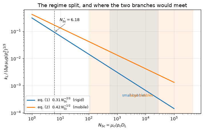
3. The small-bubble row’s diffusivity exponent
The test has a control: the same corner evaluation applied to the large-bubble row, whose printed exponent is \(-6\), using eq. (2). The control must reproduce that row’s printed \(k_L\) window without adjustment, and the test must be able to fail, which the printed \(-4\) shows it can. Both comparisons are goodness of fit (the constants were fitted to these runs); what they can see is a wrong power of ten.
r_l, r_s = RV.loc["this_work_large"], RV.loc["this_work_small"]
print(f"CONTROL  large bubbles, eq. (2), D exponent as printed ({int(r_l.D_L_exp_printed)}):")
print(f"   window / printed: bottom {A['eq2_window_lo_over_printed']:.4f}, "
      f"top {A['eq2_window_hi_over_printed']:.4f}   (printed [{r_l.kL_lo}, {r_l.kL_hi}] cm/s)")
print("\nTEST  small bubbles and rigid spheres, eq. (1): top of the window / printed top")
for e, v in A["_top"].items():
    tag = "  <- as printed" if e == int(r_s.D_L_exp_printed) else ""
    print(f"   D x 10^{e:<3d} -> {v:8.4f}{tag}")
print(f"\nThe exponent whose window top lands nearest the printed ceiling (in log distance) is "
      f"{A['small_row_exponent_selected']}, by a margin of {A['_exponent_margin']:.2f} in ln.")
print(f"Everything below uses {D_EXP_SMALL}.")
CONTROL large bubbles, eq. (2), D exponent as printed (-6):
window / printed: bottom 0.8184, top 0.8964 (printed [0.007, 0.08] cm/s)
TEST small bubbles and rigid spheres, eq. (1): top of the window / printed top
D x 10^-4 -> 21.1832 <- as printed
D x 10^-5 -> 4.5638
D x 10^-6 -> 0.9832
The exponent whose window top lands nearest the printed ceiling (in log distance) is -6, by a margin of 1.50 in ln.
Everything below uses -6.4. The packed-bed chain
Eq. (5) applied to Chu’s correlation must give the \(P/v\) the paper prints, exponent for exponent; eq. (4) with that \(P/v\) must give eq. (6); and eq. (6) at \(\Sigma = 0.41\) must give eq. (7). The chain forces the voidage group \((1-\Sigma)^{(1+a)/4}\,\Sigma^{-1}\), with \(a\) Chu’s exponent, because \(P/v\) carries \(\Sigma^{-4}\) and eq. (4) takes its fourth root; eq. (6) prints \(((1-\Sigma)/\Sigma)^{1/3}\), the same exponent on both. Three readings are carried: eq. (6) as printed, eq. (6) with \(\Sigma^{-1}\), and the chain’s own exponents.
print(f"eq. (5) + Chu -> the printed P/v: largest |ratio - 1| at two rational points "
      f"below 1e-12 (here {A['chu_identity_resid']:.1e})")
print(f"eq. (6) prefactor: {P0['c_eq4']} * {P0['c_chu']}^(1/4) = {A['eq6_prefactor_derived']:.6f}   "
      f"printed {P0['c_eq6']}   rel {A['eq6_prefactor_rel_dev']:+.2%}")
print(f"the chain's voidage and Reynolds exponent: (1 + {P0['a_chu']})/4 = {A['_chain_exp']:.2f}")
jd = A["_jd"]
print(f"\nAt Sigma = {P0['sigma_fallat']}, against the printed eq. (7) constant {P0['c_eq7']}:")
print(f"   eq. (6) as printed   j_d = {jd['printed_eq6']:.4f} Re^(-1/3)   "
      f"{A['eq7_from_printed_eq6_rel_dev']:+.1%}")
print(f"   eq. (6), Sigma^-1    j_d = {jd['sigma_inverse']:.4f} Re^(-1/3)   "
      f"{A['eq7_from_sigma_inverse_rel_dev']:+.1%}")
print(f"   the chain            j_d = {jd['chain']:.4f} Re^(-{A['_chain_exp']:.2f})")
print("Neither reading of eq. (6) reaches eq. (7). Nothing is repaired.")
re_f = A["_re_f"]
print(f"\nAgainst Fallat's measured j_d = {P0['c_fallat']} Re^({P0['e_fallat']}), largest "
      f"|deviation| over Re = {re_f[0]:,.0f} to {re_f[-1]:,.0f} ({re_f.size} points; the "
      "ratio of two power laws is monotone, so it sits at an end):")
print(f"   printed eq. (7)        {A['fallat_dev_printed_eq7']:.1%}")
print(f"   eq. (6) with Sigma^-1  {A['fallat_dev_sigma_inverse']:.1%}")
print(f"   the chain              {A['fallat_dev_chain']:.1%}")
print(f"   eq. (8), {P0['c_eq8']} Re^(-1/3)  {A['fallat_dev_eq8']:.1%}   (Fallat re-fitted at the -1/3 slope)")
print("Eq. (7) is close to Fallat, but the printed eq. (6) does not produce it, and the "
      "reading that comes nearest is a little further from Fallat.")
eq. (5) + Chu -> the printed P/v: largest |ratio - 1| at two rational points below 1e-12 (here 0.0e+00)
eq. (6) prefactor: 0.13 * 35.4^(1/4) = 0.317098 printed 0.318 rel -0.28%
the chain's voidage and Reynolds exponent: (1 + 0.44)/4 = 0.36
At Sigma = 0.41, against the printed eq. (7) constant 0.69:
eq. (6) as printed j_d = 0.3590 Re^(-1/3) -48.0%
eq. (6), Sigma^-1 j_d = 0.6505 Re^(-1/3) -5.7%
the chain j_d = 0.6396 Re^(-0.36)
Neither reading of eq. (6) reaches eq. (7). Nothing is repaired.
Against Fallat's measured j_d = 0.626 Re^(-0.322), largest |deviation| over Re = 100 to 10,000 (201 points; the ratio of two power laws is monotone, so it sits at an end):
printed eq. (7) 4.6%
eq. (6) with Sigma^-1 6.4%
the chain 28.0%
eq. (8), 0.67 Re^(-1/3) 3.6% (Fallat re-fitted at the -1/3 slope)
Eq. (7) is close to Fallat, but the printed eq. (6) does not produce it, and the reading that comes nearest is a little further from Fallat.5. The pipe chain, and the claim about it
The same machinery on the Blasius equation is the control on the packed-bed result: if the pipe chain reproduces, eq. (4)’s constant, the definition of \(j_d\) and the flow-work argument are sound, and the packed-bed problem is localised to the voidage. The paper then says eq. (9) “agrees with” Chilton-Colburn at \(N_{Re} = 10{,}000\) “with a maximum deviation of ±12 per cent” over 2000-20,000. The crossing is a root; the largest deviation is evaluated over the whole stated range.
print(f"eq. (9) prefactor: {P0['c_eq4']} * {P0['c_blasius']}^(1/4) = "
      f"{A['eq9_prefactor_derived']:.6f}   printed {P0['c_eq9']}   rel {A['eq9_prefactor_rel_dev']:+.3%}")
print(f"eq. (9) exponent : -(1/16 + 1/4) = {-(1 / 16 + 1 / 4):.4f}   printed {P0['e_eq9']}")
print(f"\nwith the printed exponent {P0['e_eq9']}:")
print(f"   crossing at N_Re = {A['pipe_cross_Re']:.0f} (the paper: {P0['re_agree_cc']:,.0f}, "
      f"{A['pipe_claim_over_cross']:.2f} times higher)")
print(f"   deviation at {P0['re_agree_cc']:,.0f}: {A['pipe_dev_at_claimed_Re']:+.2%}")
print(f"   deviation at {P0['re_lo_cc']:,.0f}: {A['_dev_lo']:+.2%},  at {P0['re_hi_cc']:,.0f}: "
      f"{A['_dev_hi']:+.2%}")
print(f"   largest |deviation| over the range {A['pipe_maxdev_over_range']:.1%} as (eq9 - CC)/CC, "
      f"{A['pipe_maxdev_paper_direction']:.1%} as (CC - eq9)/eq9")
print(f"with the exact exponent -5/16: crossing at {A['pipe_cross_Re_exact_exponent']:.0f}, "
      f"largest |deviation| {A['pipe_maxdev_over_range_exact_exponent']:.1%}")
print(f"\nThe deviation changes sign inside the stated range: "
      f"{A['pipe_deviation_changes_sign_in_range']}, so the paper's '+/-' is right about the "
      "shape; the size and the crossing are what its sentence gets wrong.")
eq. (9) prefactor: 0.13 * 0.0396^(1/4) = 0.057992 printed 0.058 rel -0.014%
eq. (9) exponent : -(1/16 + 1/4) = -0.3125 printed -0.31
with the printed exponent -0.31:
crossing at N_Re = 4480 (the paper: 10,000, 2.23 times higher)
deviation at 10,000: -8.45%
deviation at 2,000: +9.28%, at 20,000: -15.17%
largest |deviation| over the range 15.2% as (eq9 - CC)/CC, 17.9% as (CC - eq9)/eq9
with the exact exponent -5/16: crossing at 3716, largest |deviation| 17.2%
The deviation changes sign inside the stated range: True, so the paper's '+/-' is right about the shape; the size and the crossing are what its sentence gets wrong.6. Two more identities the paper’s constants must satisfy
Eq. (10), the power that just suspends solids, follows from equating eqs. (1) and (4). The paper prints its exponent structure and leaves the constant as const.; the constant is recovered here. And page 44’s \(0.31\,N_{Ra}^{1/3}\) must be eq. (1) itself.
print(f"eq. (1) = eq. (4), solved for P/v, over (g drho)^(4/3) mu^(1/3) rho^(-2/3): "
      f"parameter-free to below 1e-12 (here {A['eq10_exponent_resid']:.1e})")
print(f"   the constant the paper leaves as 'const.': ({P0['c_eq1']}/{P0['c_eq4']})^4 = "
      f"{A['eq10_implied_const']:.4f}")
print(f"eq. (1) as a Sherwood number over {P0['c_ra']} Ra^(1/3): |ratio - 1| below 1e-12 "
      f"(here {A['ra_form_resid']:.1e})")
eq. (1) = eq. (4), solved for P/v, over (g drho)^(4/3) mu^(1/3) rho^(-2/3): parameter-free to below 1e-12 (here 0.0e+00)
the constant the paper leaves as 'const.': (0.31/0.13)^4 = 32.3350
eq. (1) as a Sherwood number over 0.31 Ra^(1/3): |ratio - 1| below 1e-12 (here 0.0e+00)7. Eq. (2) against the theory it says it represents
The note added in proof says eq. (2) “represents the data of BAIRD obtained with spherical cap bubbles of equivalent diameters up to 5 cm as well as the theoretical equation proposed by this worker”, \(K_L = 0.975\,D_L^{1/2}(g/d)^{1/4}\). Eq. (2) contains no bubble diameter and Baird’s equation does, so they agree at exactly one diameter for a given liquid, computable from the two printed constants.
print("Diameter at which eq. (2) and Baird's equation coincide:")
for k, v in A["_dstar"].items():
    where = "inside" if r_l.d_lo <= v <= r_l.d_hi else ("below" if v < r_l.d_lo else "above")
    print(f"   {k:24s} d* = {v:8.4f} cm   ({where} the row's {r_l.d_lo}-{r_l.d_hi} cm)")
print(f"{A['n_baird_crossings_inside_row']} of the {len(A['_dstar'])} crossings fall inside the "
      "diameters of the large-bubble runs; across the row's viscosity range d* moves by a "
      f"factor {A['baird_cross_d_spread']:.1f}.")
print(f"At Baird's largest bubble ({P0['d_baird_max']:g} cm) in water, with D_L = "
      f"{A['_baird_DL']:.2g} cm2/s, eq. (2) stands {A['baird_ratio_at_5cm']:.2f} times above his "
      "equation.")
Diameter at which eq. (2) and Baird's equation coincide:
row minimum viscosity d* = 0.1076 cm (below the row's 0.2-0.8 cm)
water d* = 0.1357 cm (below the row's 0.2-0.8 cm)
row maximum viscosity d* = 2.3881 cm (above the row's 0.2-0.8 cm)
0 of the 3 crossings fall inside the diameters of the large-bubble runs; across the row's viscosity range d* moves by a factor 22.2.
At Baird's largest bubble (5 cm) in water, with D_L = 1.9e-06 cm2/s, eq. (2) stands 2.46 times above his equation.8. pymrm: the stagnant floor
The 2.0 of the page-44 form is the conduction limit of a sphere. The sphere is solved on a ladder of nested geometric grids; orders come from successive differences (pymrm.checks.observed_orders). The flux read at the surface and the flux read at the outer shell (times the area ratio) agree to the residual of the solve, which is the round-off scale the ladder differences are compared with.
def sphere_study(nu=2, outer="dirichlet", ns=NR_LAD, P=P0):
    """The stagnant floor on a ladder; the floor is Sh (1 - R/R_inf), its closed-form limit."""
    oo = observed_orders(lambda n: sh_sphere(RATIO, n, nu=nu, outer=outer), ns)
    floor = lambda sh: sh * (1 - RATIO)
    prod = sh_sphere(RATIO, N_R, nu=nu, outer=outer)
    shell = sh_sphere(RATIO, N_R, nu=nu, outer=outer, at="shell")
    vals = np.asarray(oo["values"])
    return {"sh_stagnant_rel_dev": floor(prod) / P["sh_floor"] - 1,
            "sh_richardson_rel_dev": abs(floor(oo["extrapolated"]) / P["sh_floor"] - 1),
            "sh_order_min": float(np.min(oo["orders"])), "sh_order_max": float(np.max(oo["orders"])),
            "sh_surface_vs_shell_flux": abs(prod / shell - 1) if shell != 0 else np.inf,
            "_finest_diff": abs(vals[-1] - vals[-2]) / abs(vals[-1]), "_oo": oo}


SPH = sphere_study()
for n, v in zip(NR_LAD, SPH["_oo"]["values"]):
    print(f"   n_r = {n:5d}   Sh(1 - R/R_inf) = {v * (1 - RATIO):.10f}   rel {v * (1 - RATIO) / 2 - 1:+.3e}")
print(f"observed orders {', '.join(f'{o:.4f}' for o in SPH['_oo']['orders'])}")
print(f"at {N_R} cells: {SPH['sh_stagnant_rel_dev']:+.2e} on the printed {P0['sh_floor']}; "
      f"Richardson limit below 1e-6 from it (here {SPH['sh_richardson_rel_dev']:.1e})")
print(f"surface flux against shell flux x area ratio: below 1e-9 "
      f"(here {SPH['sh_surface_vs_shell_flux']:.1e})")
n_r = 100 Sh(1 - R/R_inf) = 1.9954833441 rel -2.258e-03
n_r = 200 Sh(1 - R/R_inf) = 1.9989040875 rel -5.480e-04
n_r = 400 Sh(1 - R/R_inf) = 1.9997303942 rel -1.348e-04
n_r = 800 Sh(1 - R/R_inf) = 1.9999331581 rel -3.342e-05
n_r = 1600 Sh(1 - R/R_inf) = 1.9999833603 rel -8.320e-06
observed orders 2.0496, 2.0269, 2.0140
at 800 cells: -3.34e-05 on the printed 2.0; Richardson limit below 1e-6 from it (here 6.0e-08)
surface flux against shell flux x area ratio: below 1e-9 (here 3.7e-13)9. pymrm: the two branches against their closed forms
Each branch is solved at the production grid (800 cells, 800 steps) and on two ladders: the step refined at 1600 cells, and the cells refined at 800 steps. Successive differences cancel the other axis’s fixed error, so each ladder gives its own order. The Richardson limit in the step at 1600 cells still carries the cell error of 1600 cells; subtracting that error, estimated from the cell ladder, gives the two-axis limit, which is compared with the closed form. The domain truncation is negligible by construction: the Lévêque profile at 16 layer thicknesses is of order \(e^{-16^3}\), the Higbie one of order \(\operatorname{erfc}(8)\); the domain study below measures it.
def bl_study(branch, flow=None, lad=LAD, read="face", y_span=16.0, interface="dirichlet"):
    flow_, exact = BRANCH[branch]
    flow = flow_ if flow is None else flow
    run = lambda ny, nx: bl(ny, nx, read=read, y_span=y_span, interface=interface, **flow)
    prod = run(N_PROD, N_PROD)
    ox = observed_orders(lambda n: run(lad[-1], n)["kbar"], lad)
    oy = observed_orders(lambda n: run(n, N_PROD)["kbar"], lad)
    y_err = oy["values"][-1] - oy["extrapolated"]
    k_xy = ox["extrapolated"] - y_err
    return {f"{branch}_rel_err_raw": prod["kbar"] / exact - 1,
            f"{branch}_rel_err_xy_extrap": abs(k_xy / exact - 1),
            f"{branch}_x_order_min": float(np.min(ox["orders"])),
            f"{branch}_x_order_max": float(np.max(ox["orders"])),
            f"{branch}_y_order_min": float(np.min(oy["orders"])),
            f"{branch}_y_order_max": float(np.max(oy["orders"])),
            f"{branch}_balance_gap": (abs(prod["kbar"] / prod["kbar_balance"] - 1)
                                      if prod["kbar_balance"] != 0 else np.nan),
            "_finest": (min(abs(ox["values"][-1] - ox["values"][-2]),
                            abs(oy["values"][-1] - oy["values"][-2])) / abs(prod["kbar"])
                        if prod["kbar"] != 0 else np.nan),
            "_ox": ox, "_oy": oy, "_exact": exact, "_prod": prod["kbar"]}


BLS = {b: bl_study(b) for b in BRANCH}
for b, s in BLS.items():
    print(f"{b}: at {N_PROD} x {N_PROD} rel {s[f'{b}_rel_err_raw']:+.3e}; flux sum against "
          f"exit-plane balance below 1e-9 (here {s[f'{b}_balance_gap']:.1e})")
    print(f"   step ladder (n_y = {LAD[-1]}), n_x = {LAD}: rel "
          f"{', '.join(f'{v / s['_exact'] - 1:+.3e}' for v in s['_ox']['values'])}; orders "
          f"{', '.join(f'{o:.4f}' for o in s['_ox']['orders'])}")
    print(f"   cell ladder (n_x = {N_PROD}), n_y = {LAD}: rel "
          f"{', '.join(f'{v / s['_exact'] - 1:+.3e}' for v in s['_oy']['values'])}; orders "
          f"{', '.join(f'{o:.4f}' for o in s['_oy']['orders'])}")
    print(f"   two-axis limit against the closed form: below 1e-7 "
          f"(here {s[f'{b}_rel_err_xy_extrap']:.1e})")
ROUNDOFF = max(SPH["sh_surface_vs_shell_flux"], *(BLS[b][f"{b}_balance_gap"] for b in BRANCH))
FINEST_OVER_ROUNDOFF = min(SPH["_finest_diff"], *(BLS[b]["_finest"] for b in BRANCH)) / ROUNDOFF
print(f"\nsmallest last difference of any ladder over the largest two-route gap of the solves: "
      f"at least 1e3 (here {FINEST_OVER_ROUNDOFF:.1e})")
leveque: at 800 x 800 rel -1.427e-04; flux sum against exit-plane balance below 1e-9 (here 2.8e-12)
step ladder (n_y = 1600), n_x = (200, 400, 800, 1600): rel -5.562e-04, -2.787e-04, -1.398e-04, -7.041e-05; orders 0.9994, 0.9997
cell ladder (n_x = 800), n_y = (200, 400, 800, 1600): rel -2.009e-04, -1.544e-04, -1.427e-04, -1.398e-04; orders 1.9999, 2.0000
two-axis limit against the closed form: below 1e-7 (here 1.9e-08)
higbie: at 800 x 800 rel -1.600e-04; flux sum against exit-plane balance below 1e-9 (here 6.8e-12)
step ladder (n_y = 1600), n_x = (200, 400, 800, 1600): rel -6.257e-04, -3.134e-04, -1.572e-04, -7.906e-05; orders 0.9997, 0.9998
cell ladder (n_x = 800), n_y = (200, 400, 800, 1600): rel -2.164e-04, -1.713e-04, -1.600e-04, -1.572e-04; orders 1.9999, 1.9999
two-axis limit against the closed form: below 1e-7 (here 1.2e-08)
smallest last difference of any ladder over the largest two-route gap of the solves: at least 1e3 (here 4.2e+05)def domain_effect(spans=(16.0, 32.0)):
"""Relative change of the cell-extrapolated kbar when y_max goes from spans[0] to spans[1]."""
out = []
for b in BRANCH:
k = [observed_orders(lambda n: bl(n, N_PROD, y_span=s, **BRANCH[b][0])["kbar"],
(400, 800, 1600))["extrapolated"] for s in spans]
out.append(abs(k[1] / k[0] - 1))
return max(out)
DOMAIN = domain_effect()
print(f"far field moved from 16 to 32 layer thicknesses, cell-extrapolated kbar of both "
f"branches: largest relative change below 1e-8 (here {DOMAIN:.1e})")far field moved from 16 to 32 layer thicknesses, cell-extrapolated kbar of both branches: largest relative change below 1e-8 (here 8.4e-11)10. pymrm: the two exponents, and the transition between them
The exponent the paper reports is \(\mathrm d\ln k_L/\mathrm d\ln D_L\) at fixed \(u_s\), \(\dot\gamma\) and \(L\). It is computed by a central difference in \(\ln D_L\) with steps of \(\ln 1.15\), on 400 cells and 400 steps. In each pure limit the grid is scaled with the one layer thickness, so the discrete problem is self-similar and the exponents are \(2/3\) and \(1/2\) to round-off: they test the implementation, not the physics. What they catch is the wrong profile, and the break table shows they do.
The transition is not fixed by dimensional analysis. With \(\Lambda = u_s/(\dot\gamma\,\delta_{\rm Lev})\), the halfway exponent \(7/12\) and the exponent within 10 % of the mobile end (of the span \(2/3 - 1/2\)) are roots over \(\Lambda = 10^{-3}\) to \(10^{3}\). The finite-difference truncation and the grid effect on the halfway root are measured by repeating it with half the difference step and with twice the grid.
def d_ln_k_d_ln_D(u_s, gdot, n=400, rel=0.15, local=False, y_span=16.0):
    """Central difference of ln k in ln D at fixed u_s, gdot and L."""
    key = "k_local" if local else "kbar"
    k = [bl(n, n, D=D_REF * f, u_s=u_s, gdot=gdot, y_span=y_span)[key]
         for f in (1 / (1 + rel), 1 + rel)]
    return float(np.log(k[1] / k[0]) / (2 * np.log(1 + rel)))


N_HALF, N_MOBILE10 = 7 / 12, 0.5 + 0.1 * (2 / 3 - 0.5)


def transition(n=400, rel=0.15, local=False, y_span=16.0, which=("half", "mobile10")):
    expo = lambda lam: d_ln_k_d_ln_D(lam * GDOT * D_LEV, GDOT, n, rel, local, y_span)
    targets = {"half": N_HALF, "mobile10": N_MOBILE10}
    return {w: one_root(lambda lam: expo(lam) - targets[w], 1e-3, 1e3, n_scan=24, xtol=1e-8)
            for w in which}


EXP_RIGID = d_ln_k_d_ln_D(0.0, GDOT)
EXP_MOBILE = d_ln_k_d_ln_D(U_S, 0.0)
print(f"rigid  branch: d ln k / d ln D = 2/3 within 1e-9 (here {EXP_RIGID - 2 / 3:+.1e})")
print(f"mobile branch: d ln k / d ln D = 1/2 within 1e-9 (here {EXP_MOBILE - 0.5:+.1e})")

LAMS = np.array([0.0, 0.01, 0.03, 0.1, 0.2, 0.3, 0.5, 1.0, 2.0, 3.0, 10.0, 30.0, 100.0])
EXPS = np.array([d_ln_k_d_ln_D(l * GDOT * D_LEV, GDOT) for l in LAMS])
for l, e in zip(LAMS, EXPS):
    print(f"   Lambda = {l:8.3g}   d ln k / d ln D = {e:.4f}")
TR = transition()
TR_GRID = transition(n=800, which=("half",))
TR_FD = transition(rel=0.075, which=("half",))
LAM_HALF, LAM_90 = TR["half"], TR["mobile10"]
GRID_EFFECT = abs(TR_GRID["half"] / LAM_HALF - 1)
FD_EFFECT = abs(TR_FD["half"] / LAM_HALF - 1) * 4 / 3    # Richardson estimate of the O(h^2) truncation
print(f"\nhalfway (n = 7/12) at Lambda = {LAM_HALF:.5f}; within 10 % of the mobile end "
      f"(n = {N_MOBILE10:.4f}) at Lambda = {LAM_90:.4f}")
print(f"   grid: 800 cells and steps move the halfway root by below 1e-4 relative "
      f"(here {GRID_EFFECT:.1e})")
print(f"   difference step: truncation of the halfway root below 1e-4 relative "
      f"(here {FD_EFFECT:.1e})")
rigid branch: d ln k / d ln D = 2/3 within 1e-9 (here -8.4e-12)
mobile branch: d ln k / d ln D = 1/2 within 1e-9 (here +1.5e-11)
Lambda = 0 d ln k / d ln D = 0.6667
Lambda = 0.01 d ln k / d ln D = 0.6617
Lambda = 0.03 d ln k / d ln D = 0.6523
Lambda = 0.1 d ln k / d ln D = 0.6254
Lambda = 0.2 d ln k / d ln D = 0.5978
Lambda = 0.3 d ln k / d ln D = 0.5786
Lambda = 0.5 d ln k / d ln D = 0.5541
Lambda = 1 d ln k / d ln D = 0.5272
Lambda = 2 d ln k / d ln D = 0.5115
Lambda = 3 d ln k / d ln D = 0.5066
Lambda = 10 d ln k / d ln D = 0.5012
Lambda = 30 d ln k / d ln D = 0.5002
Lambda = 100 d ln k / d ln D = 0.5000
halfway (n = 7/12) at Lambda = 0.27205; within 10 % of the mobile end (n = 0.5167) at Lambda = 1.5067
grid: 800 cells and steps move the halfway root by below 1e-4 relative (here 2.6e-05)
difference step: truncation of the halfway root below 1e-4 relative (here 3.8e-05)fig, ax = plt.subplots(figsize=(6.6, 4.2))
ax.semilogx(np.where(LAMS > 0, LAMS, 1e-3), EXPS, "o-", lw=1.6, ms=4.5)
ax.axhline(2 / 3, color="tab:blue", ls="--", lw=1)
ax.axhline(0.5, color="tab:orange", ls="--", lw=1)
ax.axvline(LAM_HALF, color="0.4", ls=":", lw=1)
ax.text(1.2e-3, 2 / 3 + 0.004, r"eq. (1): $k_L\propto D^{2/3}$ (rigid)", color="tab:blue", fontsize=9)
ax.text(1.2e-3, 0.5 + 0.004, r"eq. (2): $k_L\propto D^{1/2}$ (mobile)", color="tab:orange", fontsize=9)
ax.annotate(rf"$\Lambda_{{1/2}}={LAM_HALF:.4f}$", (LAM_HALF, N_HALF), xytext=(20, -22),
textcoords="offset points", fontsize=9,
arrowprops=dict(arrowstyle="->", lw=0.8, color="0.4"))
ax.set_xlabel(r"$\Lambda = u_s\,/\,(\dot\gamma\,\delta_{\rm Lev})$ (0 = rigid; the first point is $\Lambda=0$)")
ax.set_ylabel(r"$\mathrm{d}\ln k_L/\mathrm{d}\ln D_L$")
ax.set_title("The transition the paper describes and never models")
fig.tight_layout()
plt.show()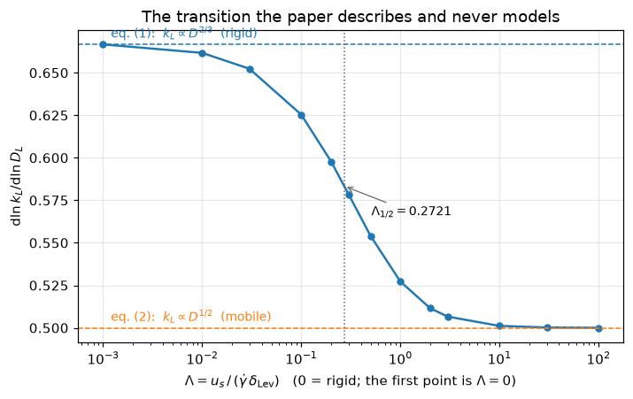
Validation
What is checked, and against what
| # | Check | Route A | Route B | What it can see |
|---|---|---|---|---|
| 1 | eq. (5) + Chu → the printed \(P/v\) | sympy on Chu as printed | the printed \(P/v\) | a mis-read constant or exponent |
| 2 | eq. (6) prefactor | \(0.13\times35.4^{1/4}\) | printed 0.318 | a mis-read constant |
| 3 | eq. (9) prefactor and exponent | \(0.13\times0.0396^{1/4}\), \(-1/16-1/4\) | printed 0.058, \(-0.31\) | a mis-read constant |
| 4 | eq. (7) from eq. (6) | two readings of the voidage group | printed 0.69 | it fails |
| 5 | eq. (9) against Chilton-Colburn | a root of the two power laws | the printed claim | it fails |
| 6, 7 | 0.28, 0.34 | Froessling × √Allen, Friedlander × \(18^{-1/3}\) | the printed predictions | a mis-read or wrong external constant |
| 8 | \(N_{Sh}\to 2\) | pymrm, nu=2, on a ladder |
printed 2.0 | the wrong geometry or outer condition |
| 9, 10 | Lévêque, Higbie magnitudes | pymrm march, two-axis limit | closed forms | the wrong profile, interface or flux read |
| 11 | exponents 2/3, 1/2 | pymrm, from solved fields | printed exponents | only a wrong profile: dimensional analysis fixes them otherwise |
| 12 | eq. (1) and page 44’s Rayleigh form | sympy | sympy | a mis-read exponent or constant |
| 13 | eq. (10) exponents | sympy on (1) and (4) | printed eq. (10) | a mis-read power |
A break row establishes sensitivity, never correctness. Every row below injects a defect and watches a claim fail, so no row can catch a baseline that is wrong rather than insensitive. That is why checks 6, 7, 9 and 10 exist: each reaches a printed or exact number by a route that shares no code with what it is compared against, and why the ladders, not the break table, bound the numerics. Nothing on this page can see whether 0.31, 0.42 and 0.13 are good fits.
Claims
Every number the page states, with how it is checked. The closed-form algebra is held to FIXED; solver results are held to SOLV. Residuals, identities and orders are bounds with their basis.
FIXED, SOLV = 1e-6, 1e-4


def value(name, x, rtol=FIXED, **kw):
    claims.value(name, x, rtol=rtol, **kw)


def bound(name, x, **kw):
    claims.bound(name, x, **kw)


# --- the two theoretical derivations --------------------------------------------------
for k in ("c28_value", "c28_rel_dev", "froessling_implied_by_paper", "froessling_implied_rel_dev",
          "allen_quarter_from_drag_law", "allen_quarter_rel_dev", "c34_value", "c34_rel_dev"):
    value(k, A[k])
claims.exact("theory_brackets_fitted", A["theory_brackets_fitted"], margin=A["_bracket_margin"],
             min_margin=0.01, note="0.276 < 0.31 < 0.340; margin the smaller relative gap")
# --- the split -----------------------------------------------------------------------------
value("crossover_Sc", A["crossover_Sc"])
value("data_sc_min_over_crossover", A["data_sc_min_over_crossover"])
claims.exact("data_sc_windows_above_crossover", A["data_sc_windows_above_crossover"],
             margin=A["_sc_margin"], min_margin=1.0,
             note="data sets whose lowest Schmidt number exceeds N_Sc*; margin relative")
value("eq2_over_eq1_large_row_sc_min", A["eq2_over_eq1_large_row_sc_min"])
value("eq2_over_eq1_large_row_sc_max", A["eq2_over_eq1_large_row_sc_max"])
for k in ("eq2_window_lo_over_printed", "eq2_window_hi_over_printed", "eq1_window_hi_over_printed",
          "eq1_window_hi_printed_exponent", "eq1_window_hi_exponent_5"):
    value(k, A[k])
claims.exact("small_row_exponent_selected", A["small_row_exponent_selected"],
             margin=A["_exponent_margin"], min_margin=0.5,
             note="log distance of the window top to the printed ceiling; margin to the runner-up")
# --- the chains ----------------------------------------------------------------------------
for k in ("eq6_prefactor_derived", "eq6_prefactor_rel_dev", "eq7_from_printed_eq6_rel_dev",
          "eq7_from_sigma_inverse_rel_dev", "fallat_dev_printed_eq7", "fallat_dev_sigma_inverse",
          "fallat_dev_chain", "fallat_dev_eq8", "eq9_prefactor_derived", "eq9_prefactor_rel_dev", "pipe_cross_Re",
          "pipe_cross_Re_exact_exponent", "pipe_claim_over_cross", "pipe_dev_at_claimed_Re",
          "pipe_maxdev_over_range", "pipe_maxdev_over_range_exact_exponent",
          "pipe_maxdev_paper_direction", "eq10_implied_const"):
    value(k, A[k])
claims.exact("pipe_deviation_changes_sign_in_range", A["pipe_deviation_changes_sign_in_range"],
             margin=A["_sign_margin"], min_margin=0.05,
             note="crossing inside 2000-20,000; margin its log distance to the nearer end over the log width")
claims.exact("pipe_maxdev_exceeds_claim", A["pipe_maxdev_exceeds_claim"],
             margin=A["_maxdev_margin"], min_margin=0.05,
             note="largest |deviation| over the stated range against 12 %; margin relative")
for k in ("chu_identity_resid", "eq10_exponent_resid", "ra_form_resid"):
    bound(k, A[k], max=1e-12, basis="identity",
          note="exact rational arithmetic at two points; nonzero only for a transcription error")
# --- Baird --------------------------------------------------------------------------------
for k in ("baird_cross_d_water_cm", "baird_cross_d_spread", "baird_ratio_at_5cm"):
    value(k, A[k])
claims.exact("n_baird_crossings_inside_row", A["n_baird_crossings_inside_row"],
             margin=A["_baird_margin"], min_margin=0.05,
             note="crossing diameters inside 0.20-0.80 cm; margin the smallest log distance to an edge")
# --- the sphere ---------------------------------------------------------------------------
value("sh_stagnant_rel_dev", SPH["sh_stagnant_rel_dev"], rtol=SOLV)
bound("sh_richardson_rel_dev", SPH["sh_richardson_rel_dev"], max=1e-6, basis="theory",
      note="Richardson limit of a second-order ladder; the next-order terms")
bound("sh_order_min", SPH["sh_order_min"], min=1.95, basis="theory", note="second order on nested geometric cells")
bound("sh_order_max", SPH["sh_order_max"], max=2.15, basis="theory", note="second order on nested geometric cells")
bound("sh_surface_vs_shell_flux", SPH["sh_surface_vs_shell_flux"], max=1e-9, basis="identity",
      note="the discrete divergence telescopes; the gap is the solve's residual")
# --- the boundary layer -------------------------------------------------------------------
for b in BRANCH:
    s = BLS[b]
    value(f"{b}_rel_err_raw", s[f"{b}_rel_err_raw"], rtol=SOLV)
    bound(f"{b}_rel_err_xy_extrap", s[f"{b}_rel_err_xy_extrap"], max=1e-7, basis="theory",
          note="two-axis Richardson limit against the closed form; next-order terms of both ladders")
    bound(f"{b}_x_order_min", s[f"{b}_x_order_min"], min=0.99, basis="theory", note="backward Euler")
    bound(f"{b}_x_order_max", s[f"{b}_x_order_max"], max=1.01, basis="theory", note="backward Euler")
    bound(f"{b}_y_order_min", s[f"{b}_y_order_min"], min=1.99, basis="theory", note="second-order cells")
    bound(f"{b}_y_order_max", s[f"{b}_y_order_max"], max=2.01, basis="theory", note="second-order cells")
    bound(f"{b}_balance_gap", s[f"{b}_balance_gap"], max=1e-9, basis="identity",
          note="backward Euler telescopes onto the boundary faces; the gap is the solves' residual")
bound("ladder_finest_over_roundoff", FINEST_OVER_ROUNDOFF, min=1e3, basis="theory",
      note="every ladder difference far above the solves' round-off")
bound("bl_domain_effect", DOMAIN, max=1e-8, basis="theory",
      note="profiles of order exp(-16^3) and erfc(8) at the far field; the rest is extrapolation residue")
bound("exp_rigid", EXP_RIGID, min=2 / 3 - 1e-9, max=2 / 3 + 1e-9, basis="identity",
      note="the grid scales with the one layer thickness: self-similar discrete problem")
bound("exp_mobile", EXP_MOBILE, min=0.5 - 1e-9, max=0.5 + 1e-9, basis="identity",
      note="the grid scales with the one layer thickness: self-similar discrete problem")
claims.count("transition_steps_decreasing", -np.diff(EXPS), 0.0, min_margin=1e-5,
             note="the exponent falls between every pair of neighbouring Lambda in the scan")
value("lambda_half", LAM_HALF, rtol=SOLV)
value("lambda_within_10pct_mobile", LAM_90, rtol=SOLV)
bound("lambda_half_grid_effect", GRID_EFFECT, max=1e-4, basis="chosen",
      note="keeps the four printed digits: 400 to 800 cells and steps")
bound("lambda_half_fd_effect", FD_EFFECT, max=1e-4, basis="chosen",
      note="keeps the four printed digits: Richardson estimate of the difference truncation")
# --- the read log ------------------------------------------------------------------------------
UNREAD = sorted(k for k in PN.index if k not in READS)
claims.exact("printed_rows_unread", ",".join(UNREAD),
             note="printed-number rows no check reads")
print(f"{len(claims.metrics)} claims registered")
76 claims registeredThe defect-injection table
Every claim above needs a row that fails its own check. The algebra claims come from algebra(P, X): each row mis-reads one printed or external constant and reruns it in full, so every claim the constant reaches is tested. A quantity that cannot be computed under a defect (a crossing that disappears) records nan, which fails its claim. The pymrm claims get rows of their own, each a call argument of the solver or the study: the geometry code, the outer and interface conditions, the velocity profile, the flux read, the far field, the grid and the ladder.
BREAK = []


def brk(row, name, broken):
    """One injected defect: ``broken`` is what claim ``name`` becomes with it."""
    if isinstance(broken, (float, np.floating)) and not np.isfinite(broken):
        broken = np.nan
    BREAK.append((row, name, claims.breaks(row, name, broken)))


def algebra_row(label, P=P0, **kw):
    """Rerun the whole algebra under one defect; register every claim it reaches."""
    a = algebra(P, **kw)
    for name in claims.metrics:
        if name in a:
            brk(label, name, a[name])


def with_(key, val):
    return Printed({**P0, key: val})


algebra_row("Chu's constant 35.4 read as 354", with_("c_chu", 354.0))
algebra_row("Chu's exponent 0.44 read as 0.50", with_("a_chu", 0.50))
algebra_row("Blasius 0.0396 read as 0.396", with_("c_blasius", 0.396))
algebra_row("eq. (4) constant 0.13 read as 0.18", with_("c_eq4", 0.18))
algebra_row("eq. (4) power 1/4 read as 1/3", eq4_power=sp.Rational(1, 3))
algebra_row("eq. (1) Schmidt exponent 2/3 read as 1/2", with_("exp_sc_eq1", 0.5))
algebra_row("eq. (2) Schmidt exponent 1/2 read as 2/3", with_("exp_sc_eq2", 2 / 3))
algebra_row("eqs (1) and (2) constants swapped", Printed({**P0, "c_eq1": P0["c_eq2"], "c_eq2": P0["c_eq1"]}))
algebra_row("page 44's 0.31 read as 0.13", with_("c_ra", 0.13))
algebra_row("Allen's 1/4 read as 1/2", with_("c_allen", 0.5))
algebra_row("Allen's drag law 10 Re^-1/2 read as 24 Re^-1/2", X={**EXT, "allen_cd": 24.0})
algebra_row("Froessling's 0.552 read as 0.525", X={**EXT, "froessling": 0.525})
algebra_row("Stokes' 18 read as 24", X={**EXT, "stokes_den": 24.0})
algebra_row("Friedlander's 0.89 read as 0.98", with_("c_friedlander", 0.98))
algebra_row("printed 0.28 read as 0.38", with_("c_froessling_allen", 0.38))
algebra_row("printed 0.34 read as 0.43", with_("c_stokes_fried", 0.43))
algebra_row("Fallat's voidage 0.41 read as 0.30", with_("sigma_fallat", 0.30))
algebra_row("eq. (6) constant 0.318 read as 0.618", with_("c_eq6", 0.618))
algebra_row("eq. (7) constant 0.69 read as 0.96", with_("c_eq7", 0.96))
algebra_row("Fallat's constant 0.626 read as 0.662", with_("c_fallat", 0.662))
algebra_row("Fallat's exponent -0.322 read as -0.222", with_("e_fallat", -0.222))
algebra_row("eq. (9) constant 0.058 read as 0.085", with_("c_eq9", 0.085))
algebra_row("eq. (9) exponent -0.31 read as -0.25", with_("e_eq9", -0.25))
algebra_row("Chilton-Colburn 0.023 read as 0.032", with_("c_cc", 0.032))
algebra_row("Chilton-Colburn exponent -0.20 read as -0.31", with_("e_cc", -0.31))
algebra_row("claimed agreement at 10,000 read as 1,000", with_("re_agree_cc", 1000.0))
algebra_row("claimed +/- 12 % read as 21 %", with_("maxdev_cc", 21.0))
algebra_row("stated range 2000-20,000 read as 200-20,000", with_("re_lo_cc", 200.0))
algebra_row("Baird's 0.975 read as 0.75", with_("c_baird", 0.75))
algebra_row("Baird's largest bubble 5 cm read as 15 cm", with_("d_baird_max", 15.0))
algebra_row("gravity in SI (9.81) in CGS formulas", X={**EXT, "g": 9.81})
algebra_row("water viscosity 1 cP entered as 1 poise", water={**WATER, "mu": 1.0})
algebra_row("small-bubble D exponent left at the printed -4", d_exp_small=-4)
_saved = set(READS)
READS.clear()
algebra(P0, skip=("baird",))
sphere_study()
brk("Baird check left out of the study", "printed_rows_unread",
    ",".join(sorted(k for k in PN.index if k not in READS)))
READS.clear()
READS.update(_saved)

# --- the sphere ---------------------------------------------------------------------------
for row, kw in (("sphere solved with nu = 0 (slab)", dict(nu=0)),
                ("sphere solved with nu = 1 (cylinder)", dict(nu=1)),
                ("sphere outer boundary closed (no flux)", dict(outer="noflux"))):
    s = sphere_study(**kw)
    for name in ("sh_stagnant_rel_dev", "sh_richardson_rel_dev", "sh_order_min", "sh_order_max",
                 "sh_surface_vs_shell_flux"):
        brk(row, name, s[name])
brk("printed floor 2.0 read as 2.2", "sh_stagnant_rel_dev",
    sphere_study(P=with_("sh_floor", 2.2))["sh_stagnant_rel_dev"])

# --- the boundary layer ------------------------------------------------------------------
def bl_row(label, branch, **kw):
    s = bl_study(branch, **kw)
    for name in claims.metrics:
        if name in s:
            brk(label, name, s[name])
    return s


_swap = {"leveque": BRANCH["higbie"][0], "higbie": BRANCH["leveque"][0]}
_rs = {}
for b in BRANCH:
    bl_row(f"{b} branch run with the other branch's velocity profile", b, flow=_swap[b])
    bl_row(f"{b} branch with a zero-flux interface", b, interface="noflux")
    _rs[b] = bl_row(f"{b} branch, flux read two-point to the first cell centre", b, read="centre")
    bl_row(f"{b} branch, far field at 2 layer thicknesses", b, y_span=2.0)
    bl_row(f"{b} ladders started at 4 cells and 4 steps", b, lad=(4, 8, 16, 32))
brk("flux read two-point to the first cell centre", "ladder_finest_over_roundoff",
    min(SPH["_finest_diff"], *(BLS[b]["_finest"] for b in BRANCH))
    / max(_rs[b][f"{b}_balance_gap"] for b in BRANCH))
brk("far field at 2 and 4 layer thicknesses", "bl_domain_effect", domain_effect((2.0, 4.0)))
brk("rigid exponent from the mobile profile", "exp_rigid", d_ln_k_d_ln_D(U_S, 0.0))
brk("mobile exponent from the rigid profile", "exp_mobile", d_ln_k_d_ln_D(0.0, GDOT))
_ex2 = np.array([d_ln_k_d_ln_D(l * GDOT * D_LEV, GDOT, y_span=0.5) for l in LAMS])
brk("transition scanned with the far field at half a layer thickness", "transition_steps_decreasing",
    int(np.sum(-np.diff(_ex2) > 0)))
_loc = transition(local=True)
brk("transition read from the local k at x = L, not the mean", "lambda_half", _loc["half"])
brk("transition read from the local k at x = L, not the mean", "lambda_within_10pct_mobile",
    _loc["mobile10"])
_g = transition(n=50, which=("half",))["half"], transition(n=100, which=("half",))["half"]
brk("grid effect measured from 50 to 100 cells", "lambda_half_grid_effect", abs(_g[1] / _g[0] - 1))
_f = transition(rel=1.0, which=("half",))["half"], transition(rel=0.5, which=("half",))["half"]
brk("difference step ln 2 instead of ln 1.15", "lambda_half_fd_effect", abs(_f[1] / _f[0] - 1) * 4 / 3)

bt = pd.DataFrame(BREAK, columns=["row", "claim", "caught"])
caught = bt[bt.caught].groupby("row", sort=False).claim.apply(list)
print(f"{len(bt.row.unique())} rows; claims each row fails:")
for row, names in caught.items():
    print(f"  {row}:")
    print("      " + ", ".join(names))
idle = [r for r in bt.row.unique() if r not in caught.index]
print(f"\nrows that fail no claim: {idle if idle else 'none'}")
missing = [n for n in claims.metrics
           if not claims.metrics[n].get("structural") and not bt[(bt.claim == n) & bt.caught].shape[0]]
print(f"claims no row fails: {missing if missing else 'none'}")
56 rows; claims each row fails:
Chu's constant 35.4 read as 354:
eq6_prefactor_derived, eq6_prefactor_rel_dev, fallat_dev_chain, chu_identity_resid
Chu's exponent 0.44 read as 0.50:
fallat_dev_chain, chu_identity_resid
Blasius 0.0396 read as 0.396:
eq9_prefactor_derived, eq9_prefactor_rel_dev, pipe_cross_Re, pipe_cross_Re_exact_exponent, pipe_claim_over_cross, pipe_dev_at_claimed_Re, pipe_maxdev_over_range, pipe_maxdev_over_range_exact_exponent, pipe_maxdev_paper_direction, pipe_deviation_changes_sign_in_range
eq. (4) constant 0.13 read as 0.18:
eq6_prefactor_derived, eq6_prefactor_rel_dev, fallat_dev_chain, eq9_prefactor_derived, eq9_prefactor_rel_dev, pipe_cross_Re, pipe_cross_Re_exact_exponent, pipe_claim_over_cross, pipe_dev_at_claimed_Re, pipe_maxdev_over_range, pipe_maxdev_over_range_exact_exponent, pipe_maxdev_paper_direction, eq10_implied_const, pipe_deviation_changes_sign_in_range
eq. (4) power 1/4 read as 1/3:
eq10_implied_const, eq10_exponent_resid
eq. (1) Schmidt exponent 2/3 read as 1/2:
crossover_Sc, data_sc_min_over_crossover, data_sc_windows_above_crossover, eq2_over_eq1_large_row_sc_min, eq2_over_eq1_large_row_sc_max, eq1_window_hi_over_printed, eq1_window_hi_printed_exponent, eq1_window_hi_exponent_5, ra_form_resid
eq. (2) Schmidt exponent 1/2 read as 2/3:
crossover_Sc, data_sc_min_over_crossover, data_sc_windows_above_crossover, eq2_over_eq1_large_row_sc_min, eq2_over_eq1_large_row_sc_max, eq2_window_lo_over_printed, eq2_window_hi_over_printed, baird_cross_d_water_cm, baird_cross_d_spread, baird_ratio_at_5cm
eqs (1) and (2) constants swapped:
theory_brackets_fitted, crossover_Sc, data_sc_min_over_crossover, eq2_over_eq1_large_row_sc_min, eq2_over_eq1_large_row_sc_max, eq2_window_lo_over_printed, eq2_window_hi_over_printed, eq1_window_hi_over_printed, eq1_window_hi_printed_exponent, eq1_window_hi_exponent_5, eq10_implied_const, ra_form_resid, baird_cross_d_water_cm, baird_ratio_at_5cm, n_baird_crossings_inside_row
page 44's 0.31 read as 0.13:
ra_form_resid
Allen's 1/4 read as 1/2:
c28_value, c28_rel_dev, froessling_implied_by_paper, froessling_implied_rel_dev, allen_quarter_rel_dev, theory_brackets_fitted
Allen's drag law 10 Re^-1/2 read as 24 Re^-1/2:
allen_quarter_from_drag_law, allen_quarter_rel_dev
Froessling's 0.552 read as 0.525:
c28_value, c28_rel_dev, froessling_implied_rel_dev
Stokes' 18 read as 24:
c34_value, c34_rel_dev, theory_brackets_fitted
Friedlander's 0.89 read as 0.98:
c34_value, c34_rel_dev
printed 0.28 read as 0.38:
c28_rel_dev, froessling_implied_by_paper, froessling_implied_rel_dev
printed 0.34 read as 0.43:
c34_rel_dev
Fallat's voidage 0.41 read as 0.30:
eq7_from_printed_eq6_rel_dev, eq7_from_sigma_inverse_rel_dev, fallat_dev_sigma_inverse, fallat_dev_chain
eq. (6) constant 0.318 read as 0.618:
eq6_prefactor_rel_dev, eq7_from_printed_eq6_rel_dev, eq7_from_sigma_inverse_rel_dev, fallat_dev_sigma_inverse
eq. (7) constant 0.69 read as 0.96:
eq7_from_printed_eq6_rel_dev, eq7_from_sigma_inverse_rel_dev, fallat_dev_printed_eq7
Fallat's constant 0.626 read as 0.662:
fallat_dev_printed_eq7, fallat_dev_sigma_inverse, fallat_dev_chain, fallat_dev_eq8
Fallat's exponent -0.322 read as -0.222:
fallat_dev_printed_eq7, fallat_dev_sigma_inverse, fallat_dev_chain, fallat_dev_eq8
eq. (9) constant 0.058 read as 0.085:
eq9_prefactor_rel_dev
eq. (9) exponent -0.31 read as -0.25:
pipe_cross_Re, pipe_claim_over_cross, pipe_dev_at_claimed_Re, pipe_maxdev_over_range, pipe_maxdev_paper_direction, pipe_deviation_changes_sign_in_range
Chilton-Colburn 0.023 read as 0.032:
pipe_cross_Re, pipe_cross_Re_exact_exponent, pipe_claim_over_cross, pipe_dev_at_claimed_Re, pipe_maxdev_over_range, pipe_maxdev_over_range_exact_exponent, pipe_maxdev_paper_direction, pipe_deviation_changes_sign_in_range
Chilton-Colburn exponent -0.20 read as -0.31:
pipe_cross_Re, pipe_cross_Re_exact_exponent, pipe_claim_over_cross, pipe_dev_at_claimed_Re, pipe_maxdev_over_range, pipe_maxdev_over_range_exact_exponent, pipe_maxdev_paper_direction, pipe_deviation_changes_sign_in_range
claimed agreement at 10,000 read as 1,000:
pipe_claim_over_cross, pipe_dev_at_claimed_Re
claimed +/- 12 % read as 21 %:
pipe_maxdev_exceeds_claim
stated range 2000-20,000 read as 200-20,000:
pipe_maxdev_over_range, pipe_maxdev_over_range_exact_exponent, pipe_maxdev_paper_direction
Baird's 0.975 read as 0.75:
baird_cross_d_water_cm, baird_ratio_at_5cm
Baird's largest bubble 5 cm read as 15 cm:
baird_ratio_at_5cm
gravity in SI (9.81) in CGS formulas:
eq2_window_lo_over_printed, eq2_window_hi_over_printed, eq1_window_hi_over_printed, eq1_window_hi_printed_exponent, eq1_window_hi_exponent_5, small_row_exponent_selected, baird_cross_d_water_cm, baird_ratio_at_5cm, n_baird_crossings_inside_row
water viscosity 1 cP entered as 1 poise:
baird_cross_d_water_cm, baird_ratio_at_5cm
small-bubble D exponent left at the printed -4:
data_sc_min_over_crossover, data_sc_windows_above_crossover, eq1_window_hi_over_printed
Baird check left out of the study:
printed_rows_unread
sphere solved with nu = 0 (slab):
sh_stagnant_rel_dev, sh_richardson_rel_dev, sh_order_min, sh_order_max, sh_surface_vs_shell_flux
sphere solved with nu = 1 (cylinder):
sh_stagnant_rel_dev, sh_richardson_rel_dev, sh_surface_vs_shell_flux
sphere outer boundary closed (no flux):
sh_stagnant_rel_dev, sh_richardson_rel_dev, sh_order_min, sh_order_max, sh_surface_vs_shell_flux
printed floor 2.0 read as 2.2:
sh_stagnant_rel_dev
leveque branch run with the other branch's velocity profile:
leveque_rel_err_raw, leveque_rel_err_xy_extrap
leveque branch with a zero-flux interface:
leveque_rel_err_raw, leveque_rel_err_xy_extrap, leveque_x_order_min, leveque_x_order_max, leveque_y_order_min, leveque_y_order_max, leveque_balance_gap
leveque branch, flux read two-point to the first cell centre:
leveque_rel_err_raw, leveque_balance_gap
leveque branch, far field at 2 layer thicknesses:
leveque_rel_err_raw
leveque ladders started at 4 cells and 4 steps:
leveque_rel_err_xy_extrap, leveque_x_order_min, leveque_y_order_min
higbie branch run with the other branch's velocity profile:
higbie_rel_err_raw, higbie_rel_err_xy_extrap
higbie branch with a zero-flux interface:
higbie_rel_err_raw, higbie_rel_err_xy_extrap, higbie_x_order_min, higbie_x_order_max, higbie_y_order_min, higbie_y_order_max, higbie_balance_gap
higbie branch, flux read two-point to the first cell centre:
higbie_rel_err_raw, higbie_rel_err_xy_extrap, higbie_y_order_min, higbie_balance_gap
higbie branch, far field at 2 layer thicknesses:
higbie_rel_err_raw, higbie_rel_err_xy_extrap
higbie ladders started at 4 cells and 4 steps:
higbie_rel_err_xy_extrap, higbie_x_order_min, higbie_y_order_min, higbie_y_order_max
flux read two-point to the first cell centre:
ladder_finest_over_roundoff
far field at 2 and 4 layer thicknesses:
bl_domain_effect
rigid exponent from the mobile profile:
exp_rigid
mobile exponent from the rigid profile:
exp_mobile
transition scanned with the far field at half a layer thickness:
transition_steps_decreasing
transition read from the local k at x = L, not the mean:
lambda_half, lambda_within_10pct_mobile
grid effect measured from 50 to 100 cells:
lambda_half_grid_effect
difference step ln 2 instead of ln 1.15:
lambda_half_fd_effect
rows that fail no claim: none
claims no row fails: noneWhich printed constants the checks read
Computed from the read log of the printed-number dictionary, not asserted.
print(f"{len(PN) - len(UNREAD)} of {len(PN)} printed-number rows are read by a check.")
print("Rows no check reads:")
for k in UNREAD:
    print(f"   {k:<18} {PN.loc[k, 'quantity']}  (printed {PN.loc[k, 'printed_value']})")
print(f"\nThe large-bubble row of the Range of Variables table starts at d = "
      f"{r_l.d_lo} cm, below the printed split of {PN.loc['d_split', 'printed_value']} cm: "
      "the split is corroborated by the diameter columns but tested by nothing here.")
30 of 33 printed-number rows are read by a check.
Rows no check reads:
d_split bubble diameter separating "small" from "large" (printed 0.25)
fig6_span span of the variables covered by Fig. 6 (printed 10000000.0)
sd_eq4 standard deviation of the Fig. 6 regression (printed 66.0)
The large-bubble row of the Range of Variables table starts at d = 0.2 cm, below the printed split of 0.25 cm: the split is corroborated by the diameter columns but tested by nothing here.What pymrm adds
The transition is turned into a number. The paper describes it three times (Fig. 3’s intermediate-size bubbles, deep pools driving large-bubble coefficients down to rigid-sphere values, and “surface active agents cause the high mass transfer coefficients for large bubbles to be reduced to those obtained with rigid spheres”) and models it nowhere. All three say the interface stops moving. Written as \(u(y) = u_s + \dot\gamma y\), one group \(\Lambda = u_s/(\dot\gamma\,\delta_{\rm Lev})\) controls it, the exponent \(\mathrm d\ln k_L/\mathrm d\ln D_L\) falls at every step of the scan from \(2/3\) to \(1/2\), and the halfway point is a root. The paper’s two correlations are the two ends of that one curve. pymrm supplies the operators of the two linear problems (the spherical shell and the marched layer) and the flux reads; the rest of the page, the paper’s own algebra, is NumPy and sympy and owes pymrm nothing.
The boundary layer does not predict the constants. It reproduces the exponents and the interpolation between them, which is the mechanism claim. The prefactors 0.31 and 0.42 absorb bubble shape, slip velocity, swarm hindrance and the interfacial-area definition, none of which a flat interface of contact length \(L\) contains.
print(f"halfway at Lambda = {LAM_HALF:.4f}; within 10 % of the mobile end by Lambda = {LAM_90:.3f}")
print(f"the scan falls at {claims['transition_steps_decreasing']} of {LAMS.size - 1} steps")
halfway at Lambda = 0.2721; within 10 % of the mobile end by Lambda = 1.507
the scan falls at 12 of 12 stepsReuse
Take the correlation. Eqs. (1) and (2) are two lines of code and need no solver. The rule for choosing between them, in the paper’s own terms: bubbles below about 2½ mm, or any interface contaminated by surface-active material, or a deep pool where a large bubble has had time to accumulate a skin: eq. (1); clean, freshly formed bubbles above 2½ mm in a shallow pool: eq. (2). Both of the paper’s data sets sit far above the crossover \(N_{Sc}^\star\) (section 2), so in a liquid the choice matters.
Do not read eq. (2) as size-independent outside its window: section 7 shows where it and Baird’s equation coincide, and how far that diameter moves with the viscosity.
Take the boundary-layer solver. BoundaryLayer in model.py is the generic convection-diffusion layer over a moving or rigid wall: change u_s and gdot for a different interface mobility, or give u another profile (it is built once with construct_coefficient_matrix). It is S4 machinery marched in space rather than time, as S2 does for a plug-flow reactor. A reacting solute makes the problem nonlinear and needs newton per step.
Take the exponent diagnostic. d_ln_k_d_ln_D tells which transport mechanism a model is in: differentiate its output with respect to the diffusivity and look at the number.
Related pages. A3.3 (Danckwerts surface renewal) solves the penetration limit this page’s mobile branch reduces to; the two are not independent confirmations of each other, and this page checks against the closed form \(2\sqrt{D u_s/\pi L}\), not against A3.3. A3.1 (Whitman two-film) supplies the resistance-in-series bookkeeping that turns a \(k_L\) from here into an overall coefficient. A3.4 (Wakao-Funazkri) is the packed-bed Sherwood correlation; for a packed bed use it, not eq. (7), for the reason in section 4.
What to be careful with. Eq. (4)’s 66 % standard deviation is not a typo for 6.6 %: a correlation with that scatter is an order-of-magnitude tool. Eq. (7) should not be used. The ±12 % claim about eq. (9) does not hold as stated. The small-bubble row of the Range of Variables table has a wrong power of ten on \(D_L\), and two further rows of the same column are unusable.
print(f"Runtime (here {time.time() - T_START:.0f} s)")
# Claims: prints every registered number, writes agreement.json for CI, and
# raises when a claim fails its own check or has no break row.
claims.report();   # the semicolon keeps the notebook from echoing the payload
Runtime (here 31 s)
Claims for A3.6:
c28_value = 0.276 value rtol 1e-06
c28_rel_dev = -0.014286 value rtol 1e-06
froessling_implied_by_paper = 0.56 value rtol 1e-06
froessling_implied_rel_dev = 0.014493 value rtol 1e-06
allen_quarter_from_drag_law = 0.26099 value rtol 1e-06
allen_quarter_rel_dev = 0.043965 value rtol 1e-06
c34_value = 0.3396 value rtol 1e-06
c34_rel_dev = -0.0011807 value rtol 1e-06
theory_brackets_fitted = True exact exact, margin 0.0872
crossover_Sc = 6.1848 value rtol 1e-06
data_sc_min_over_crossover = 17.121 value rtol 1e-06
data_sc_windows_above_crossover = 2 exact exact, margin 16.1
eq2_over_eq1_large_row_sc_min = 2.9469 value rtol 1e-06
eq2_over_eq1_large_row_sc_max = 11.895 value rtol 1e-06
eq2_window_lo_over_printed = 0.81842 value rtol 1e-06
eq2_window_hi_over_printed = 0.89635 value rtol 1e-06
eq1_window_hi_over_printed = 0.98324 value rtol 1e-06
eq1_window_hi_printed_exponent = 21.183 value rtol 1e-06
eq1_window_hi_exponent_5 = 4.5638 value rtol 1e-06
small_row_exponent_selected = -6 exact exact, margin 1.5
eq6_prefactor_derived = 0.3171 value rtol 1e-06
eq6_prefactor_rel_dev = -0.002835 value rtol 1e-06
eq7_from_printed_eq6_rel_dev = -0.47968 value rtol 1e-06
eq7_from_sigma_inverse_rel_dev = -0.057218 value rtol 1e-06
fallat_dev_printed_eq7 = 0.046184 value rtol 1e-06
fallat_dev_sigma_inverse = 0.063834 value rtol 1e-06
fallat_dev_chain = 0.27998 value rtol 1e-06
fallat_dev_eq8 = 0.0358 value rtol 1e-06
eq9_prefactor_derived = 0.057992 value rtol 1e-06
eq9_prefactor_rel_dev = -0.00014009 value rtol 1e-06
pipe_cross_Re = 4479.9 value rtol 1e-06
pipe_cross_Re_exact_exponent = 3716.4 value rtol 1e-06
pipe_claim_over_cross = 2.2322 value rtol 1e-06
pipe_dev_at_claimed_Re = -0.08454 value rtol 1e-06
pipe_maxdev_over_range = 0.15175 value rtol 1e-06
pipe_maxdev_over_range_exact_exponent = 0.17249 value rtol 1e-06
pipe_maxdev_paper_direction = 0.17889 value rtol 1e-06
eq10_implied_const = 32.335 value rtol 1e-06
pipe_deviation_changes_sign_in_range = True exact exact, margin 0.35
pipe_maxdev_exceeds_claim = True exact exact, margin 0.265
chu_identity_resid = (here 0.0e+00) bound bound <= 1e-12 [identity]
eq10_exponent_resid = (here 0.0e+00) bound bound <= 1e-12 [identity]
ra_form_resid = (here 0.0e+00) bound bound <= 1e-12 [identity]
baird_cross_d_water_cm = 0.13566 value rtol 1e-06
baird_cross_d_spread = 22.185 value rtol 1e-06
baird_ratio_at_5cm = 2.4639 value rtol 1e-06
n_baird_crossings_inside_row = 0 exact exact, margin 0.388
sh_stagnant_rel_dev = -3.3421e-05 value rtol 0.0001
sh_richardson_rel_dev = (here 6.0e-08) bound bound <= 1e-06 [theory]
sh_order_min = (here 2.0e+00) bound bound >= 1.95 [theory]
sh_order_max = (here 2.0e+00) bound bound <= 2.15 [theory]
sh_surface_vs_shell_flux = (here 3.7e-13) bound bound <= 1e-09 [identity]
leveque_rel_err_raw = -0.00014275 value rtol 0.0001
leveque_rel_err_xy_extrap = (here 1.9e-08) bound bound <= 1e-07 [theory]
leveque_x_order_min = (here 1.0e+00) bound bound >= 0.99 [theory]
leveque_x_order_max = (here 1.0e+00) bound bound <= 1.01 [theory]
leveque_y_order_min = (here 2.0e+00) bound bound >= 1.99 [theory]
leveque_y_order_max = (here 2.0e+00) bound bound <= 2.01 [theory]
leveque_balance_gap = (here 2.8e-12) bound bound <= 1e-09 [identity]
higbie_rel_err_raw = -0.00016 value rtol 0.0001
higbie_rel_err_xy_extrap = (here 1.2e-08) bound bound <= 1e-07 [theory]
higbie_x_order_min = (here 1.0e+00) bound bound >= 0.99 [theory]
higbie_x_order_max = (here 1.0e+00) bound bound <= 1.01 [theory]
higbie_y_order_min = (here 2.0e+00) bound bound >= 1.99 [theory]
higbie_y_order_max = (here 2.0e+00) bound bound <= 2.01 [theory]
higbie_balance_gap = (here 6.8e-12) bound bound <= 1e-09 [identity]
ladder_finest_over_roundoff = (here 4.2e+05) bound bound >= 1000 [theory]
bl_domain_effect = (here 8.4e-11) bound bound <= 1e-08 [theory]
exp_rigid = (here 6.7e-01) bound bound [0.666667, 0.666667] [identity]
exp_mobile = (here 5.0e-01) bound bound [0.5, 0.5] [identity]
transition_steps_decreasing = 12 exact exact, margin 0.000187
lambda_half = 0.27205 value rtol 0.0001
lambda_within_10pct_mobile = 1.5067 value rtol 0.0001
lambda_half_grid_effect = (here 2.6e-05) bound bound <= 0.0001 [chosen]
lambda_half_fd_effect = (here 3.8e-05) bound bound <= 0.0001 [chosen]
printed_rows_unread = 'd_split,fig6_span,sd_eq4' exact exact