# Bootstrap: the pymrm this page was checked with, and the gallery files it was
# published with. Works in a checkout, in CI and on a fresh Colab VM.
GALLERY_REF = "gallery-2026.11.10.3"  # replaced by the release tag at publication
PYMRM = ">=3.4.0,<4"  # equals meta.yaml pymrm_min_version, up to the next major
PAGE = "A3.5-ranz-marshall-froessling"  # equals the page directory

import os, sys, urllib.request
from pathlib import Path
_shared = next((p / "shared" for p in (Path.cwd(), *Path.cwd().parents)
                if (p / "shared" / "gallery_bootstrap.py").is_file()), None)
if _shared is None:
    _shared = (Path(os.environ.get("XDG_CACHE_HOME") or Path.home() / ".cache")
               / "pymrm-gallery" / GALLERY_REF)
    _shared.mkdir(parents=True, exist_ok=True)
    urllib.request.urlretrieve(
        "https://raw.githubusercontent.com/computational-chemical-engineering/"
        f"pymrm-gallery/{GALLERY_REF}/shared/gallery_bootstrap.py",
        _shared / "gallery_bootstrap.py")
sys.path.insert(0, str(_shared))
sys.modules.pop("gallery_bootstrap", None)
from gallery_bootstrap import setup
setup(PAGE, PYMRM, GALLERY_REF); # the semicolon stops the cell echoing the pathRanz-Marshall: the only constant this paper tests is the 2.0, and the authors’ own water data miss it
sec:A
struct:S3
tier:T0
data:tier3
phase:gas-liquid
Nu = 2 + 0.6 Re^(1/2) Pr^(1/3) as Ranz and Marshall published it in 1952, taken apart constant by constant. The 0.60 is fitted to the very tables any comparison uses; the 1/2 and 1/3 are Froessling’s, assumed and not testable from the transcribed tables; the 2.0 is the one piece of theory. Extrapolated to zero Reynolds number, the paper’s heat and benzene runs are consistent with 2.0 and its water mass-transfer runs fall three standard errors below it. The authors saw the gap and named its likeliest cause; this page puts a number on it, against the claim in their abstract to have verified the intercept. pymrm recomputes the 2.0 from the spherical BVP it comes from, and confirms the closed form that sizes the radial-convection factor Ranz said in 1993 the papers had underplayed.
Ranz-Marshall: the only constant this paper tests is the 2.0
Catalog ID: A3.5 · Structures: S3 (pointwise algebra, plus a 1-D spherical BVP) · Tier: T0
\[N_{Nu} = 2.0 + 0.60\,N_{Pr}^{1/3}N_{Re}^{1/2}, \qquad N_{Nu}' = 2.0 + 0.60\,N_{Sc}^{1/3}N_{Re}^{1/2}\]
Two of the most-used equations in chemical engineering, and they contain four numbers with four different epistemic statuses:
| constant | status in the papers |
|---|---|
2.0 |
theoretical. Part I derives it (eq. 7) from the conduction/diffusion field around a sphere at rest. Nothing was fitted. |
0.60 |
fitted, to Figures 6, 7 and 9, that is, to Tables 1, 2, 3 and 4, the same tables anyone would compare against. |
1/2 |
assumed. Froessling’s boundary-layer form, carried over. |
1/3 |
assumed. Same, and not identifiable from Tables 1–4, every run of which is in air. Part II tests it graphically in Figure 12, which this page does not digitise. |
So a page that reports “the correlation reproduces the paper’s data to a few per cent” has reported a goodness of fit and nothing else. This page keeps the four apart and asks what the data can actually decide.
What comes out. The intercept is the only testable constant, and the paper’s data test it three separate ways: an outcome the paper reports in words rather than in numbers. Extrapolated to \(N_{Re}=0\) by a free two-parameter fit, with the standard error of the intercept from the fit’s own scatter, Table 1’s heat-transfer runs give 2.0582 ± 0.0538 (+2.9 %, 1.1 standard errors above 2.0) and Table 4’s benzene mass-transfer runs 2.0523 ± 0.1245 (+2.6 %, 0.4 standard errors): both consistent with the theoretical 2.0. Table 1’s water mass-transfer runs give 1.7322 ± 0.0870, -13.4 %, 3.1 standard errors below it, beyond the two-sided 5 % point of Student’s t. The still-air row says the same thing more bluntly: it prints \(N_{Nu}=2.23\) and \(N_{Nu}'=1.79\) for a situation in which eqs. (21) and (22) both say 2.0, a ratio of 1.2458 where the correlation demands exactly 1.
The authors saw this, and said so, qualitatively. Part II, folio 173, first column:
“The points for heat transfer extrapolate close to the theoretical minimum value. Experimental values obtained for \(N_{Nu}\) at \(N_{Re} = 0\) were slightly greater than 2.0, and the small difference is attributed to free convection. … Data for mass transfer show a steeper slope and a lower intercept, but the disagreement is always less than 10 per cent at a given \(N_{Re}\) and is usually much less than 5 per cent. Factors which may have contributed to errors in the data and anomalies in the heat- and mass-transfer analogy were: (1) inaccurate values of diffusivity; (2) \(p_{Ai}\) may not have been the saturation vapor pressure; (3) the partial pressure of water vapor in the air may not have been zero at low air rates …”
So the direction, and the cause this page finds most consistent with the numbers, are the authors’ own. What is added here is the arithmetic they did not do, and it changes what the sentence means:
- the deficit is -13.4 % on the intercept, not “less than 10 per cent”: their bound is about the curves at a given \(N_{Re}\), where the fitted 0.60 absorbs most of it, not about the extrapolated intercept;
- 3.1 standard errors of the fitted intercept, so it is not “small”;
- it is species-specific: benzene, whose diffusivity came from Hirschfelder, Bird and Spotz rather than from the authors’ own Figure 5, lands where the heat data land; only water misses;
- \(N_{Nu}'\propto 1/D_v\), so closing the water gap needs a diffusivity smaller by 1.117, which is exactly the 0.204 sq.cm/sec Part II prints, and calls “a low value compared with other methods of determination”.
And that puts the numbers against two claims the papers do make. Part I’s abstract says the study “confirmed the analogy between heat and mass transfer at low Reynolds numbers, and verified the simple expression for the Nusselt number at zero Reynolds number”, while the paper’s own still-air pair has an analogy ratio of 1.2458. Folio 174 says the correlation’s success carries “an implication that the calculated value of the diffusivity of water vapor in air may be more accurate than any reported in the literature”, while the same data, read at the intercept, say that diffusivity is 1.117 too large. The gap is not an oversight of the authors’. The published conclusions drawn from it are what these numbers sit against.
And pymrm. The 2.0 is a boundary-value problem, so it is computed here rather than quoted: a spherical shell with construct_div(nu=2), one linear solve per grid on a ladder of nested grids, second order, whose Richardson limit lies below 1e-6 from the exact 2. The same solver, with construct_convflux_upwind added, answers the question Ranz raised in 1993 about the radial-convection factor, and shows which of the two readings of the paper’s own definition of \(p_f\) is the right one.
Background
Ranz and Marshall published “Evaporation from Drops” in two parts in Chemical Engineering Progress 48 in 1952, out of W. R. Marshall’s spray-drying programme at Wisconsin. One drop, about a millimetre across, hangs from a microburet in an upward air stream; liquid is fed in fast enough to hold the diameter constant, and the feed rate is the evaporation rate. A 0.5-mil thermocouple inside the drop gives its temperature. That is the whole experiment, and it is why the paper is still read: it is a single-particle measurement in a field that otherwise had to infer transfer coefficients from beds and sprays.
The page-range discrepancy, recorded both ways. Part I’s scan frames carry two folio lines, one above the black edge of the leaf, one inside it at the foot, differing by exactly two. Four of the six frames show both legibly (139/141, 140/142, 141/143 and 144/146); on the fourth frame the upper line is cut off at the leaf edge and on the fifth there is no upper line at all, so those two pairs are inferred from the sequence rather than read. Part II settles which belongs to the page: its first page has a blank top margin and prints Vol. 48, No. 4 | Chemical Engineering Progress | Page 173 at the foot of the text block. In this issue the folio is a footer. The line at the top of a Part I frame is therefore the preceding leaf’s footer, caught in the same frame, and Part I’s own folios are 141–146, which is the universal citation and the one Ranz himself gives in his 1993 ISI Citation Classic (“Chem. Eng. Progr. 48:141-6; 173-80, 1952”). The 139–144 reading on file comes from reading the upper line as a running head. Every page reference on this page is the folio printed at the foot of the page the value appears on. Part II is 173–180 either way.
Neither file has a text layer at all (pdftotext returns one byte per page), so every digit here was read off 400 dpi renders (the files’ native resolution: pdfimages -list reports JPEG RGB tiles at 400 × 400 ppi, so rendering larger only interpolates), with each numeric column cropped and magnified on its own.
Two files on disk are not this paper and are named here so nobody re-opens them hoping: MISC-Ranz1993-citation-classic-commentary-CurrContents22.pdf is a one-page 1993 reminiscence carrying none of the correlations, and Charlesworth1960-evaporation-drops-dissolved-solids-AIChEJ6-9.pdf is a companion study about crust formation in drops containing dissolved solids. The 1993 file is quoted once on this page, for a caveat only its author could give.
The published model
Part I, eq. (7): the theory. With the fluid at rest (\(v_\theta = v_r = 0\)), eqs. (1), (2), (5) and (6) collapse to
\[N_{Nu} = N_{Nu}' = 2.0. \tag{7}\]
That is steady conduction (or diffusion) from a sphere into an unbounded stagnant medium, and it is the only piece of the correlation that is derived.
Part I, eqs. (8) and (9): the form, from Froessling.
\[N_{Nu}' = 2.0 + K_1 (N_{Sc})^m (N_{Re})^n, \qquad N_{Nu} = 2.0 + K_2 (N_{Pr})^p (N_{Re})^q\]
with, in the paper’s own words, “\(K_1 = K_2\), \(p = m = 1/3\), and \(q = n = 1/2\).” Ranz went to Pittsburgh to read the only copy of Froessling’s 1938 paper in the United States and translated it himself (he tells that story in the 1993 commentary, not in the papers); the exponents are Froessling’s, adopted here, not measured here.
Part II, eqs. (21) and (22): the constant.
\[N_{Nu} = 2.0 + 0.60\,N_{Pr}^{1/3}N_{Re}^{1/2}, \qquad N_{Nu}' = 2.0 + 0.60\,N_{Sc}^{1/3}N_{Re}^{1/2}\]
Part II, eq. (24), and a constant the papers do not flag as such.
\[h = h_c = \frac{k}{D_p}\left(2.0 + 0.54\,N_{Re}^{1/2}\right), \qquad\text{"restricted to aqueous drops".}\]
0.54 is 0.60 times \(Pr^{1/3}\) for air, so the three printed numbers together pin the Prandtl number the authors used: \((0.54/0.60)^3\) = 0.729. That is a definition, not a check: nothing independent is compared with it, and nothing can be, because this page’s own rule forbids importing a property value. It is worth having anyway: it means the whole heat-transfer analysis can be done without importing one.
How the Nusselt numbers were measured (Part I, eqs. 16, 19, 20). At finite velocity from the feed rate; in still air from the slope of \(D_p^2\) against time,
\[N_{Nu} = -\tfrac14\frac{\lambda_v\rho_l}{\Delta t\,k}\frac{\mathrm{d}D_p^2}{\mathrm{d}\tau}, \qquad N_{Nu}' = -\tfrac14\frac{\rho_l M_m p_f}{\Delta p_A D_v \rho_{gm}}\frac{\mathrm{d}D_p^2}{\mathrm{d}\tau}.\]
The \(p_f\) in that second expression is the object Ranz singled out forty-one years later, and Part II’s notation defines it only as the “average value of \((\pi - p_A)\) across transfer path”, without saying which average. The validation section settles it.
Parameters and assumptions
Theirs. Quasi-steady transfer around an isolated sphere; the drop surface at a single temperature \(t_i\) and saturated at \(p_{Ai} = p_{Ai}(t_i)\); the transfer path of uniform temperature and velocity; the drop spherical (Part II notes the diameter along the capillary axis was about 8 % greater than across it, and \(D_p\) is the arithmetic mean of the two); radiation, sensible heat of the feed and conduction along the capillary removed as corrections (Part I eq. 18); no thermal diffusion or Dufour effect (“negligible in this study”).
Ours. Nothing added. Every transfer number used here is the paper’s own \(N_{Nu}\), \(N_{Nu}'\) and \(N_{Re}\) column; no property of air, water or benzene is imported from outside the two papers, and the one Prandtl number that appears is back-calculated from the paper’s own eq. (24). The pymrm sections use a unit diffusivity and a unit sphere, because both answers are dimensionless.
What is out of scope, and why. Figures 5 (transport properties), 12 (the five-decade master correlation), 13 (free convection) and 14 (vapour pressure over NH₄NO₃ solutions) carry content that exists only as curves. No maintainer figure review is available for this case, so no point is read off any of them and no number on this page comes from one. Figure 12 is named twice below, once for what its printed legend lists and once for the sentence on folio 174 that comments on it; that is reading type, not reading a curve, and nothing numerical follows from it. Three consequences are stated rather than worked around: the free-convection exponent \(1/4\) of eqs. (10) and (11) is never exercised on this page, because the only zero-Reynolds datum in any table is the single still-air row; Table 6’s calculated evaporation rates cannot be reproduced, because they need the vapour-pressure curve of Figure 14; and the paper’s own test of the Prandtl exponent, which lives entirely in Figure 12, is neither reproduced nor contradicted here. Table 5 (drop temperature against Reynolds number) is not used either: it carries no transfer coefficient.
The data
Five files, all transcribed from the papers’ own tables: tier 3, table transcription, no digitisation anywhere.
| file | what it is | rows |
|---|---|---|
…-table1.csv |
Part II Table 1, water drops in dry air, folio 174 | 18 forced + 1 still-air |
…-table2.csv |
Part II Table 2, water drops in 66–90 °C air, folio 175 | 9 |
…-table3.csv |
Part II Table 3, water drops in 85–221 °C air, from the motion-picture record, folio 175 | 9 |
…-table4.csv |
Part II Table 4, benzene drops, folio 176 | 13 |
…-printed-constants.csv |
every constant either part prints, with its role | 24 |
Four things about these rows that the analysis has to respect.
- The 0.60 was fitted to all of them. Figures 6, 7 and 9 are exactly Tables 1–4. There is no held-out set for the correlation anywhere in either part, and this page never claims one: where it needs an out-of-range test it refits the coefficient on Table 1’s room-temperature runs alone and then applies it to Table 3. (There is a held-out set for the reference-temperature convention: Table 3 again, which prints no Reynolds column and so cannot enter that fit. It is used below, and its scope is stated where it is used.)
- Three \(N_{Nu}'\) cells are unreadable. An ink blot on the microfilm covers the mass-transfer entries of Table 1 runs 12, 13 and 14. They are left empty, not guessed; the mass-transfer fits use the 15 rows that remain, and the break table shows what filling them in by eye would do.
- One digit in Table 4 is settled by arithmetic, not by the glyph. Run 11’s \(N_{Nu}'\) is degraded on the film. It is recorded as 10.0, and the reason is in the mass-transfer cell below: both of Table 4’s transfer numbers come from the same measured rate, so their ratio depends only on the printed temperatures and pressure, and the neighbouring rows bracket run 11 tightly enough to exclude every other reading, including the 10.6 that the glyph’s counter position alone would suggest.
- Table 4 has no corrected \(N_{Nu}\) column at all, because for benzene the sensible-heat term is about 20 % of the heat flow and the authors did not attempt one. Apparent and corrected Nusselt numbers are never mixed on this page.
The Reynolds column is the transcription check, and it turns out to be more than that. The tables define \(N_{Re} = D_p v_o\rho/\mu\) and print \(D_p\), \(v_o\), the air and drop temperatures and the pressure beside it, so it is over-determined: every printed Reynolds number with a measured drop temperature (the cell below prints the count) must lie on one \(\rho/\mu(T,P)\) law. Neither part says at what temperature the air properties in those columns were evaluated. The one place either part states a reference temperature is for the single still-air run, and that statement is reconciled below with what the columns give; so the next cell leaves \(T_{\rm ref}\) as an unknown and lets those rows answer it.
import numpy as np
import pandas as pd
import matplotlib.pyplot as plt
from scipy.integrate import quad
from scipy.optimize import curve_fit, minimize_scalar
from scipy.stats import t as student_t
from pymrm.checks import find_roots, observed_orders
from gallery_utils import load_data, load_meta, cite_data, Claims
from model import (nu_shell, sh_stefan, sh_closed, pf_log, pf_arith, corr_excess,
                   stefan_threshold, stefan_threshold_lambertw)

plt.rcParams.update({"figure.dpi": 110, "axes.grid": True, "grid.alpha": 0.3})
claims = Claims(PAGE.split("-")[0])
A = {}                                 # every computed number the claims read
print("environment ready")
environment readyTABLES = {f"t{i}": f"ranz-marshall-1952-table{i}.csv" for i in (1, 2, 3, 4)}
D0 = {k: load_data(f, page=PAGE) for k, f in TABLES.items()}
# the same tables as printed strings, for the rounding half-widths (a trailing zero
# is a printed digit)
D0.update({k + "s": load_data(f, page=PAGE, dtype=str) for k, f in TABLES.items()})
K = load_data("ranz-marshall-1952-printed-constants.csv", page=PAGE).set_index("quantity")
KS = load_data("ranz-marshall-1952-printed-constants.csv", page=PAGE, dtype=str).set_index("quantity")
print(cite_data(load_meta("ranz-marshall-1952-table1.csv", page=PAGE)), "\n")
def split(D, n_re=0.5):
"""The still-air row, the forced-convection rows of Table 1, Table 4, and the
rows with a readable N_Nu'. ``sqRe`` is N_Re to the Reynolds exponent."""
t1 = D["t1"]
still = t1[t1.run == 19].iloc[0]
t1f = t1[t1.run != 19].copy()
t4 = D["t4"].copy()
t1f["sqRe"] = t1f.Re.to_numpy() ** n_re
t4["sqRe"] = t4.Re.to_numpy() ** n_re
return still, t1f, t4, t1f.Nu_prime.notna().to_numpy()
def half_unit(s):
"""Half a unit in the last printed place of the decimal string ``s``."""
s = str(s).strip()
return 0.5 * 10.0 ** (-(len(s.split(".")[1]) if "." in s else 0))
# The still-air row is not a forced-convection run and never joins a regression.
still, t1f, t4, mass_ok = split(D0)
t2, t3 = D0["t2"], D0["t3"]
print(f"Table 1: {len(t1f)} forced-convection runs, Re {t1f.Re.min():g} to {t1f.Re.max():g}, "
f"plus one still-air row")
print(f" mass-transfer column usable on {mass_ok.sum()} of {len(t1f)} "
f"(ink damage on runs {list(t1f.run[~mass_ok])})")
print(f"Table 2: {len(t2)} runs, air {t2.air_temp_C.min():g}-{t2.air_temp_C.max():g} C")
print(f"Table 3: {len(t3)} rows, air {t3.air_temp_C.min():g}-{t3.air_temp_C.max():g} C, "
f"abscissa printed")
print(f"Table 4: {len(t4)} benzene runs, Re {t4.Re.min():g} to {t4.Re.max():g}")
print(f"still air: N_Nu = {still.Nu_apparent:g}, N_Nu' = {still.Nu_prime:g}, "
f"P = {still.press_mmHg:g} mm Hg")Ranz, W. E.; Marshall, W. R., Jr. (1952) — Chemical Engineering Progress 48(4) 173-180 (April 1952), 'Evaporation from Drops, Part II' — table
Table 1: 18 forced-convection runs, Re 2.11 to 195, plus one still-air row
mass-transfer column usable on 15 of 18 (ink damage on runs [12, 13, 14])
Table 2: 9 runs, air 66.4-90 C
Table 3: 9 rows, air 85-221 C, abscissa printed
Table 4: 13 benzene runs, Re 3.7 to 220
still air: N_Nu = 2.23, N_Nu' = 1.79, P = 741 mm HgThe constants, with their roles
# Every printed constant, by its name in the CSV. Every function below takes this
# dictionary, so a misread constant is one call (the break table does exactly that).
P0 = {k: float(K.loc[k, "value"]) for k in K.index}

print(K[["value", "role"]].to_string(), "\n")
print("roles:", dict(K.role.value_counts()))


def pr_implied(P):
    """Eq. (24) collapses eqs. (21) for air: 0.54 = 0.60 Pr^(1/3) fixes the Prandtl
    number the authors used. A DEFINITION, not a check: nothing independent is
    compared with it, because the page imports no property value."""
    return (P["aqueous_collapsed_coefficient"] / P["correlation_coefficient_K"]) ** (
        1.0 / P["exponent_Pr_Sc"])


def nu_corr(Re, P):
    """Eq. (24), the aqueous collapsed form 2.0 + 0.54 Re^(1/2)."""
    return (P["correlation_intercept"]
            + P["aqueous_collapsed_coefficient"] * np.asarray(Re, float) ** P["exponent_Re"])


def nu_from_abscissa(X, P, Kc=None):
    """Eq. (21) on the paper's own printed abscissa N_Re^(1/2) N_Pr^(1/3)."""
    Kc = P["correlation_coefficient_K"] if Kc is None else Kc
    return P["correlation_intercept"] + Kc * np.asarray(X, float)


def pct(model, data):
    model, data = np.asarray(model, float), np.asarray(data, float)
    return 100.0 * (model - data) / data


def rms_pct(model, data):
    return float(np.sqrt(np.mean(pct(model, data) ** 2)))


A["pr_air_implied_by_eq24"] = pr_implied(P0)
print(f"\neq. (24)'s {P0['aqueous_collapsed_coefficient']:g} against eqs. (21)'s "
      f"{P0['correlation_coefficient_K']:g} with the printed 1/3 exponent")
print(f"  => the Prandtl number of air the authors used: {A['pr_air_implied_by_eq24']:.5f}")
print("  (a DEFINITION, not an agreement: it is (0.54/0.60)^3 and this page never")
print("   compares it with a tabulated Prandtl number, because importing one is")
print("   exactly what the page refuses to do.)")
value role
quantity
correlation_intercept 2.000000 theoretical
correlation_coefficient_K 0.600000 fitted
exponent_Pr_Sc 0.333333 assumed
exponent_Re 0.500000 assumed
exponent_Gr_free_convection 0.250000 assumed
freeconv_coefficient 0.600000 fitted
aqueous_collapsed_coefficient 0.540000 derived
stillair_Nu_measured 2.230000 measured
stillair_Nuprime_measured 1.790000 measured
Dv_backed_out_cm2_s 0.204000 derived
Dv_backout_temperature_K 290.000000 measured
Dv_backout_pressure_mmHg 741.000000 measured
test80_Nu_apparent 5.830000 measured
test80_correction_sensible_heat 0.028000 derived
test80_correction_radiation 0.006000 derived
test80_correction_capillary 0.011000 derived
test80_Nu_corrected 5.570000 derived
eq19_eq20_prefactor 0.250000 derived
k_water_20C_cal_s_cm_C 0.001430 measured
k_water_over_k_air 25.000000 measured
benzene_melting_point_F 42.000000 measured
table6_Re 66.600000 measured
table6_Dp_cm 0.106000 measured
table3_pressure_mmHg 743.000000 measured
roles: {'measured': np.int64(11), 'derived': np.int64(7), 'assumed': np.int64(3), 'fitted': np.int64(2), 'theoretical': np.int64(1)}
eq. (24)'s 0.54 against eqs. (21)'s 0.6 with the printed 1/3 exponent
=> the Prandtl number of air the authors used: 0.72900
(a DEFINITION, not an agreement: it is (0.54/0.60)^3 and this page never
compares it with a tabulated Prandtl number, because importing one is
exactly what the page refuses to do.)The transcription check
A single two-parameter law \(\rho/\mu = C\,P\,T_{\rm ref}^{\,n}\) against every printed Reynolds number in Tables 1, 2 and 4 that has a measured drop temperature, with the reference temperature written \(T_{\rm ref} = T_a + w\,(T_d - T_a)\) and \(w\) left free. Then a nearly fit-free companion: nine rows of Table 1 sit at one pressure inside 0.7 °C of each other in air temperature, so their nine \(Re/v\) values are very nearly one number, and the cell says how nearly, because nearly is the whole content of the check.
# The Reynolds column is over-determined by the columns beside it: the tables
# define N_Re = D_p v rho / mu and print D_p, v, air temperature and pressure, so
# Re/(D_p v P) is a function of temperature alone. Fit
#     ln( Re / (D_p v P) ) = c0 + c1 ln T_ref
# and look at the residuals. A misread digit cannot hide there. But WHICH T_ref?
# Neither part states the convention for the TABLES. (Part II states one for the
# single still-air run, "an average temperature of 290 deg K.", and that statement
# is reconciled with the recovered value at the end of this cell.) So the reference
# temperature is left as an unknown weight w between the air and the drop:
#     T_ref = T_air + w (T_drop - T_air),   w = 0 free stream, w = 1/2 film, w = 1 drop.
def re_frame(df):
    d = df[(df.Re > 0) & df.drop_temp_C.notna()]
    return pd.DataFrame({"D": d.D_p_cm, "v": d.air_vel_cm_s, "Ta": d.air_temp_C,
                         "Td": d.drop_temp_C, "P": d.press_mmHg, "Re": d.Re})


def re_data(D):
    """Every row of Tables 1, 2 and 4 with a measured drop temperature, and ln(Re/(D v P))."""
    R = pd.concat([re_frame(D["t1"]).assign(tab=1), re_frame(D["t2"]).assign(tab=2),
                   re_frame(D["t4"]).assign(tab=4)], ignore_index=True)
    return R, np.log(R.Re / (R.D * R.v * R.P)).to_numpy()


def t_ref(F, w):
    return (F.Ta + w * (F.Td - F.Ta) + 273.15).to_numpy()


def re_fit(w, R, y):
    """Least squares of y on [1, ln T_ref(w)]: exponent, its standard error, residuals."""
    X = np.column_stack([np.ones(len(y)), np.log(t_ref(R, w))])
    c, *_ = np.linalg.lstsq(X, y, rcond=None)
    r = y - X @ c
    se = float(np.sqrt(np.sum(r ** 2) / (len(y) - 2) * np.linalg.inv(X.T @ X)[1, 1]))
    return float(c[1]), se, r


def re_rms(w, R, y):
    return float(np.sqrt(np.mean(re_fit(w, R, y)[2] ** 2)))


def d_ssr_dw(w, R, y):
    """Exact derivative of the residual sum of squares in w. The coefficients are
    optimal at every w, so only the explicit dependence counts:
    dSSR/dw = -2 c1 sum(r (T_d - T_a)/T_ref)."""
    c1, _, r = re_fit(w, R, y)
    return float(-2.0 * c1 * np.sum(r * (R.Td - R.Ta).to_numpy() / t_ref(R, w)))


def reynolds(D, P, w=None, band=1.05):
    """The rho/mu law, its reference temperature, and the checks that hang on it."""
    still, t1f, _, _ = split(D, P["exponent_Re"])
    R, y = re_data(D)
    if w is None:
        # the minimum of the rms over w is the root of the exact derivative on [0, 1]
        roots = find_roots(lambda ww: d_ssr_dw(ww, R, y), 0.0, 1.0, n_scan=64)["roots"]
        roots = [r for r in roots if re_rms(r, R, y) < min(re_rms(0.0, R, y), re_rms(1.0, R, y))]
        w = float(roots[0]) if len(roots) == 1 else np.nan
    out = {"_R": R, "_y": y, "_w": w}
    n_best, se_best, r_best = re_fit(w, R, y) if np.isfinite(w) else (np.nan, np.nan, y * np.nan)
    n_air, se_air, r_air = re_fit(0.0, R, y)
    out.update(re_reference_temperature_weight=w, re_law_T_exponent=n_best,
               re_law_T_exponent_se=se_best,
               re_law_resid_rms_pct=float(100 * np.sqrt(np.mean(r_best ** 2))),
               re_law_resid_max_pct=float(100 * np.max(np.abs(r_best))),
               re_law_resid_rms_pct_free_stream=float(100 * np.sqrt(np.mean(r_air ** 2))),
               re_law_T_exponent_free_stream=n_air, _se_air=se_air, _r_best=r_best)
    # the band of w within 5 % of the best rms: the two roots of rms(w) = 1.05 rms(w*)
    target = band * np.sqrt(np.mean(r_best ** 2))
    edges = find_roots(lambda ww: re_rms(ww, R, y) - target, 0.0, 1.0, n_scan=64)["roots"]
    lo, hi = (edges if len(edges) == 2 else (np.nan, np.nan))
    out.update(re_reference_weight_band=float(hi - lo), _lo=lo, _hi=hi,
               re_band_holds_045_and_055=bool(lo < 0.45 and hi > 0.55),
               _band_margin=float(min(0.45 - lo, hi - 0.55)) if np.isfinite(lo) else np.nan)
    # every row's N_Re re-evaluated at the free stream instead of at T_ref(w)
    ratio = ((R.Ta + 273.15).to_numpy() / t_ref(R, w)) ** n_best
    nu_now, nu_alt = nu_corr(R.Re.to_numpy(), P), nu_corr(R.Re.to_numpy() / ratio, P)
    out.update(re_freestream_worst_Re_pct=float(100 * np.max(np.abs(1 / ratio - 1))),
               re_freestream_worst_Nu_pct=float(100 * np.max(np.abs(nu_alt / nu_now - 1))))
    # nine rows of Table 1 at one pressure: Re/v is nearly one number
    iso = t1f[t1f.press_mmHg == 738]
    r_v = (iso.Re / iso.air_vel_cm_s).to_numpy()
    rm_iso = t_ref(pd.DataFrame({"Ta": iso.air_temp_C, "Td": iso.drop_temp_C}), w) ** n_best
    s1 = D["t1s"].set_index("run").loc[iso.run.astype(str)]
    hw = 100 * np.array([half_unit(a) / float(a) + half_unit(b) / float(b)
                         for a, b in zip(s1.Re, s1.air_vel_cm_s)])
    spread = float(100.0 * np.ptp(r_v) / r_v.mean())
    t_eff = float(100.0 * np.ptp(rm_iso) / rm_iso.mean())
    rnd = float(np.sort(hw)[-1] + np.sort(hw)[-2])      # a peak-to-peak bound: two rows
    out.update(t1_iso_Re_over_v_spread_pct=spread, t1_iso_expected_spread_from_T_pct=t_eff,
               t1_iso_rounding_ptp_bound_pct=rnd, _iso=iso, _r_v=r_v, _hw=hw,
               _T_iso=t_ref(pd.DataFrame({"Ta": iso.air_temp_C, "Td": iso.drop_temp_C}), w),
               t1_iso_spread_below_T_effect=bool(spread < t_eff),
               _iso_margin=abs(t_eff - spread) / spread,
               t1_iso_spread_inside_T_plus_rounding=bool(spread < t_eff + rnd),
               _iso_margin2=abs(t_eff + rnd - spread) / spread)
    # the one reference temperature Part II states, for the still-air run
    T_film = float(still.air_temp_C + 0.5 * (still.drop_temp_C - still.air_temp_C) + 273.15)
    out.update(stillair_film_minus_stated_K=T_film - P["Dv_backout_temperature_K"],
               _T_film=T_film, _still=still)
    return out


RE = reynolds(D0, P0)
A.update({k: v for k, v in RE.items() if not k.startswith("_")})
R_ALL, Y_ALL, W = RE["_R"], RE["_y"], RE["_w"]

print(f"{len(R_ALL)} printed Reynolds numbers (every row with a measured drop")
print("temperature) against one rho/mu = C P T_ref^n law.\n")
print(f"  {'w':>6}{'reference temperature':>24}{'exponent n':>13}{'+-':>8}"
      f"{'rms':>9}{'worst':>9}")
for w, lab in ((0.0, "air (free stream)"), (1/3, "one-third film"),
               (0.5, "film (mean)"), (1.0, "drop surface")):
    n_, se_, r_ = re_fit(w, R_ALL, Y_ALL)
    print(f"  {w:6.3f}{lab:>24}{n_:13.3f}{se_:8.3f}"
          f"{100*np.sqrt(np.mean(r_**2)):8.3f} %{100*np.max(np.abs(r_)):8.3f} %")

print(f"\n  the minimum, a root of the exact derivative dSSR/dw on [0, 1]: w = {W:.4f},")
print(f"  the arithmetic mean of the air and drop temperatures to {abs(W-0.5)/0.5*100:.2f} %.")
print(f"  There the exponent is {A['re_law_T_exponent']:+.3f} +- {A['re_law_T_exponent_se']:.3f} "
      f"(n = {len(R_ALL)}, {len(R_ALL) - 2} dof),")
print("  what kinetic theory gives for air (mu ~ T^0.7 and rho ~ P/T give n ~ -1.7); at the")
print(f"  free stream it is {A['re_law_T_exponent_free_stream']:+.3f} +- {RE['_se_air']:.3f}, "
      f"{abs((A['re_law_T_exponent_free_stream'] + 1.7) / RE['_se_air']):.0f} standard errors away")
print(f"  from it. The residual falls from {A['re_law_resid_rms_pct_free_stream']:.3f} % "
      f"to {A['re_law_resid_rms_pct']:.3f} %.")
print(f"  The band of w within 5 % of the best residual (two roots) is "
      f"[{RE['_lo']:.3f}, {RE['_hi']:.3f}],")
print(f"  width {A['re_reference_weight_band']:.3f}: the film rule is identified, but a 0.45 or")
print(f"  a 0.55 rule lies inside the band too ({A['re_band_holds_045_and_055']}).")
print("\n  THE PAPERS DO NOT STATE THIS CONVENTION FOR THE TABLES; it is recovered")
print("  here from the printed columns alone, and it matters downstream.")
print("  Re-evaluating every row's Reynolds number at the free stream instead of")
print(f"  the film shifts it by up to {A['re_freestream_worst_Re_pct']:.1f} %, and the N_Nu "
      f"that eq. (24)")
print(f"  then predicts by up to {A['re_freestream_worst_Nu_pct']:.1f} %. See Reuse.")
_r = RE["_r_best"]
for tab in (1, 2, 4):
    sel = (R_ALL.tab == tab).to_numpy()
    print(f"    Table {tab}: {sel.sum():2d} rows, rms "
          f"{100*np.sqrt(np.mean(_r[sel]**2)):.3f} %, worst "
          f"{100*np.max(np.abs(_r[sel])):.3f} %")
worst_i = int(np.argmax(np.abs(_r)))       # names the row; the value is the metric above
print(f"  worst single row: Table {R_ALL.tab[worst_i]}, v = {R_ALL.v[worst_i]:g} cm/s, "
      f"Re = {R_ALL.Re[worst_i]:g}, off by {100*_r[worst_i]:+.2f} %")
print("  (Table 2's runs 1-4 are excluded throughout: they print no drop temperature,")
print("   the table's own note saying adiabatic saturation was assumed instead.)")

# A NEARLY fit-free version of the same check. Table 1's runs 6-14 share a pressure
# and sit inside 0.7 C of each other in air temperature, so their nine Re/v values
# are very nearly one number. Not exactly one number: their DROP temperatures spread
# the film temperature over about 1 K, which at the fitted exponent is a real
# effect of its own. And the quantity being bounded is a nine-row peak-to-peak, so
# the bound it is compared with is a peak-to-peak bound, the two largest half-widths.
iso = RE["_iso"]
print(f"\nTable 1 runs {iso.run.min()}-{iso.run.max()} (all 738 mm Hg, "
      f"{iso.air_temp_C.min()}-{iso.air_temp_C.max()} C air): Re/v = {RE['_r_v'].mean():.5f}")
print(f"  observed peak-to-peak spread            {A['t1_iso_Re_over_v_spread_pct']:6.3f} %")
print(f"  film temperature moves over these rows  "
      f"{RE['_T_iso'].min():.2f}-{RE['_T_iso'].max():.2f} K, which at n = "
      f"{A['re_law_T_exponent']:.3f} is")
print(f"  a real spread in rho/mu of              {A['t1_iso_expected_spread_from_T_pct']:6.3f} %")
print(f"  rounding alone allows, peak-to-peak,    {A['t1_iso_rounding_ptp_bound_pct']:6.3f} %  "
      f"(worst single row +-{RE['_hw'].max():.3f} %)")
print(f"  observed spread below the temperature effect alone: "
      f"{A['t1_iso_spread_below_T_effect']}; inside temperature plus rounding: "
      f"{A['t1_iso_spread_inside_T_plus_rounding']}.")
print("  So this is NOT a reference-temperature-free check. What it is, is a")
print("  gross-transcription detector: a misread digit in Re or v shows up as a")
print("  single outlier, and the break table exercises exactly that.")

# WHAT THE PAPER ITSELF SAYS ABOUT THE REFERENCE TEMPERATURE. Part II states the
# convention once, for the still-air run: D_v = 0.204 sq.cm./sec. "at an average
# temperature of 290 deg K." Table 1's still-air row prints the air and the drop
# temperature that go with it, so the two can be reconciled.
T_STATED, P_STATED = P0["Dv_backout_temperature_K"], P0["Dv_backout_pressure_mmHg"]
print(f"\n  AND THE PAPER STATES IT ONCE ITSELF. Part II gives D_v = "
      f"{P0['Dv_backed_out_cm2_s']:g} sq.cm/sec")
print(f"  'at an average temperature of {T_STATED:g} deg K. and a pressure of "
      f"{P_STATED:g} mm. Hg.'")
print(f"  Table 1's still-air row prints air {still.air_temp_C:g} C and drop "
      f"{still.drop_temp_C:g} C at {still.press_mmHg:g} mm Hg.")
print(f"    free stream        {still.air_temp_C + 273.15:7.2f} K")
print(f"    film (w = 1/2)     {RE['_T_film']:7.2f} K   <- the authors' 'average'")
print(f"    drop surface       {still.drop_temp_C + 273.15:7.2f} K")
print(f"    stated             {T_STATED:7.2f} K,  difference from the film "
      f"{A['stillair_film_minus_stated_K']:+.2f} K")
print(f"  and the stated pressure equals the row's own printed pressure: "
      f"{P_STATED == still.press_mmHg}.")
print(f"  So w = {W:.4f} is not only a minimisation: for the one run where the")
print("  authors say which average they took, they took the film temperature.")
36 printed Reynolds numbers (every row with a measured drop
temperature) against one rho/mu = C P T_ref^n law.
w reference temperature exponent n +- rms worst
0.000 air (free stream) -1.323 0.033 1.141 % 3.301 %
0.333 one-third film -1.587 0.027 0.787 % 2.544 %
0.500 film (mean) -1.766 0.027 0.695 % 2.463 %
1.000 drop surface -2.569 0.121 2.102 % 3.882 %
the minimum, a root of the exact derivative dSSR/dw on [0, 1]: w = 0.4996,
the arithmetic mean of the air and drop temperatures to 0.08 %.
There the exponent is -1.765 +- 0.027 (n = 36, 34 dof),
what kinetic theory gives for air (mu ~ T^0.7 and rho ~ P/T give n ~ -1.7); at the
free stream it is -1.323 +- 0.033, 11 standard errors away
from it. The residual falls from 1.141 % to 0.695 %.
The band of w within 5 % of the best residual (two roots) is [0.405, 0.582],
width 0.178: the film rule is identified, but a 0.45 or
a 0.55 rule lies inside the band too (True).
THE PAPERS DO NOT STATE THIS CONVENTION FOR THE TABLES; it is recovered
here from the printed columns alone, and it matters downstream.
Re-evaluating every row's Reynolds number at the free stream instead of
the film shifts it by up to 15.5 %, and the N_Nu that eq. (24)
then predicts by up to 5.4 %. See Reuse.
Table 1: 18 rows, rms 0.126 %, worst 0.288 %
Table 2: 5 rows, rms 1.374 %, worst 2.462 %
Table 4: 13 rows, rms 0.767 %, worst 2.045 %
worst single row: Table 2, v = 17.6 cm/s, Re = 9, off by -2.46 %
(Table 2's runs 1-4 are excluded throughout: they print no drop temperature,
the table's own note saying adiabatic saturation was assumed instead.)
Table 1 runs 6-14 (all 738 mm Hg, 24.3-25.0 C air): Re/v = 0.62789
observed peak-to-peak spread 0.492 %
film temperature moves over these rows 289.11-290.06 K, which at n = -1.765 is
a real spread in rho/mu of 0.578 %
rounding alone allows, peak-to-peak, 0.612 % (worst single row +-0.385 %)
observed spread below the temperature effect alone: True; inside temperature plus rounding: True.
So this is NOT a reference-temperature-free check. What it is, is a
gross-transcription detector: a misread digit in Re or v shows up as a
single outlier, and the break table exercises exactly that.
AND THE PAPER STATES IT ONCE ITSELF. Part II gives D_v = 0.204 sq.cm/sec
'at an average temperature of 290 deg K. and a pressure of 741 mm. Hg.'
Table 1's still-air row prints air 24.9 C and drop 9.1 C at 741 mm Hg.
free stream 298.05 K
film (w = 1/2) 290.15 K <- the authors' 'average'
drop surface 282.25 K
stated 290.00 K, difference from the film +0.15 K
and the stated pressure equals the row's own printed pressure: True.
So w = 0.4996 is not only a minimisation: for the one run where the
authors say which average they took, they took the film temperature.The residual is smallest at \(w\) = 0.4996, a root of the exact derivative of the residual sum of squares, i.e. the arithmetic mean of the air and the drop temperatures. That is not a small preference. At the film temperature the fitted exponent is -1.765 ± 0.027, what kinetic theory gives for air, since \(\mu\sim T^{0.7}\) and \(\rho\sim P/T\) make \(\rho/\mu\sim P\,T^{-1.7}\), and the residual over all rows is 0.69 %; at the free stream the exponent is -1.32, many of its standard errors from \(-1.7\) (the count is printed above), and the residual is 1.14 %. Table 1’s own rows come back to the per-table rms and worst printed above once the film temperature is used: four-figure Reynolds numbers reproduced from four other printed columns by a two-parameter law.
And the papers state it once themselves, for the one run where they had to. Part II’s still-air paragraph gives \(D_v = 0.204\) sq.cm/sec “at an average temperature of 290° K. and a pressure of 741 mm. Hg.” Table 1’s still-air row prints the air and drop temperatures that go with it, and their mean is 0.15 K above the stated value, with the stated pressure equal to the row’s own printed pressure. So for the single run whose reference temperature the authors write down, the average they took is the film temperature. The recovered \(w\) is not only a minimisation; it agrees with the one printed statement of the convention in either part.
That leaves the tables’ convention genuinely unstated (no part says at what temperature the Reynolds columns of Tables 1, 2 and 4 were evaluated), and it carries into anyone’s reuse of the correlation: evaluating \(N_{Re}\) at the free stream instead of the film would move it by up to 15.5 % on these very rows, and the \(N_{Nu}\) that eq. (24) then predicts by up to 5.4 %.
The identification has a width and the page states it: the band of \(w\) within 5 % of the best residual, between the two roots of rms\((w) = 1.05\,\)rms\((w^*)\), is 0.178 wide, so a \(0.45\) or a \(0.55\) rule would not be distinguishable from \(1/2\). What is distinguishable is the free stream, and the drop surface.
The \(Re/v\) check needs a reference temperature too. Nine rows at one pressure and one air temperature do not give one number: their drop temperatures spread the film temperature over about a kelvin, which at the fitted exponent is a 0.578 % effect on \(\rho/\mu\), on its own larger than the whole 0.492 % spread observed. And the observed quantity is a nine-row peak-to-peak, so the bound it must be judged against is a peak-to-peak bound, 0.612 % from rounding alone (the two largest half-widths), not one row’s half-width. Read that way the check passes comfortably and is a gross-transcription detector, not a reference-temperature-free identity.
The convention has an out-of-sample test, on rows the fit could not see
Table 3 prints no Reynolds column at all, so none of its rows can enter the fit above. It does print \(D_p\), \(v\), both temperatures and (in its footnote) the pressure, so the recovered law can be asked to predict the abscissa Table 3 does print, at reference temperatures above every one the law was fitted on (both ranges are printed below).
# THE FIT HAS AN OUT-OF-SAMPLE TEST. Table 3 prints NO Reynolds column at all,
# only the abscissa N_Re^(1/2) N_Pr^(1/3), so not one of its rows can enter the fit
# above, which used the rows of Tables 1, 2 and 4. But it prints D_p, v, the air
# and drop temperatures, and its footnote prints the pressure, so the recovered law
# can PREDICT its abscissa and be scored against the printed one, at reference
# temperatures beyond every one the law was fitted on.
def t3_abscissa(w, D, P, R, y):
    """Table 3's abscissa predicted from the rho/mu law refitted at this w."""
    d3 = D["t3"]
    c = np.polyfit(np.log(t_ref(R, w)), y, 1)                 # [slope, intercept]
    T3 = t_ref(pd.DataFrame({"Ta": d3.air_temp_C, "Td": d3.drop_temp_C}), w)
    Re3 = (np.exp(c[1]) * T3 ** c[0] * d3.D_p_corresponding_cm.to_numpy()
           * d3.air_vel_cm_s.to_numpy() * P["table3_pressure_mmHg"])
    return Re3 ** P["exponent_Re"] * pr_implied(P) ** P["exponent_Pr_Sc"]


def t3_rms(w, D, P, R, y):
    return rms_pct(t3_abscissa(w, D, P, R, y), D["t3"].Re_half_Pr_third.to_numpy())


W_SCAN = np.linspace(0.0, 1.0, 101)


def table3_heldout(D, P, w, R, y):
    """Table 3 scored at the recovered w, at both ends, and its own best w: a scan of
    101 points over [0, 1], refined by a bounded minimisation between the neighbours
    of the smallest scan value."""
    s = np.array([t3_rms(ww, D, P, R, y) for ww in W_SCAN])
    i = int(np.argmin(s))
    if i in (0, len(W_SCAN) - 1):
        best = np.nan                       # at or beyond the end of [0, 1]
    else:
        best = float(minimize_scalar(lambda ww: t3_rms(ww, D, P, R, y),
                                     bounds=(W_SCAN[i - 1], W_SCAN[i + 1]), method="bounded",
                                     options={"xatol": 1e-10}).x)
    T_fit = t_ref(R, w)
    T_t3 = t_ref(pd.DataFrame({"Ta": D["t3"].air_temp_C, "Td": D["t3"].drop_temp_C}), w)
    return {"t3_heldout_rms_pct": t3_rms(w, D, P, R, y) if np.isfinite(w) else np.nan,
            "t3_extrapolation_K": float(T_t3.max() - T_fit.max()), "_T": (T_fit, T_t3),
            "t3_heldout_rms_pct_free_stream": t3_rms(0.0, D, P, R, y),
            "t3_heldout_rms_pct_drop_surface": t3_rms(1.0, D, P, R, y),
            "t3_heldout_w": best}


TH = table3_heldout(D0, P0, W, R_ALL, Y_ALL)
A.update({k: v for k, v in TH.items() if not k.startswith("_")})
T_fit, T_t3 = TH["_T"]
print(f"reference temperatures the law was FITTED on : "
      f"{T_fit.min():.1f} - {T_fit.max():.1f} K  ({len(R_ALL)} rows)")
print(f"reference temperatures Table 3 asks it about : "
      f"{T_t3.min():.1f} - {T_t3.max():.1f} K  ({len(t3)} rows, NONE in the fit)")
print(f"  the two ranges overlap: {T_t3.min() <= T_fit.max()}; the extrapolation reaches "
      f"{A['t3_extrapolation_K']:.0f} K beyond the fit.\n")

X3p = t3.Re_half_Pr_third.to_numpy()
print(f"  {'w':>6}{'reference temperature':>24}{'Table 3 abscissa rms':>22}{'worst':>10}")
for w, lab in ((0.0, "air (free stream)"), (W, "the RECOVERED value"), (1.0, "drop surface")):
    r_ = pct(t3_abscissa(w, D0, P0, R_ALL, Y_ALL), X3p)
    print(f"  {w:6.3f}{lab:>24}{np.sqrt(np.mean(r_**2)):19.3f} %{np.max(np.abs(r_)):9.3f} %")
print(f"\n  and the w that best reproduces Table 3 ON ITS OWN (scan of {len(W_SCAN)} points "
      f"on [0, 1], refined) is {A['t3_heldout_w']:.4f},")
print(f"  against the {W:.4f} recovered from the other three tables. This is a test of")
print("  the reference-temperature convention only: the 0.60 was fitted to Table 3")
print("  (Figure 9), so nothing here is out of sample for the CORRELATION.")
reference temperatures the law was FITTED on : 280.8 - 329.1 K (36 rows)
reference temperatures Table 3 asks it about : 330.4 - 409.7 K (9 rows, NONE in the fit)
the two ranges overlap: False; the extrapolation reaches 81 K beyond the fit.
w reference temperature Table 3 abscissa rms worst
0.000 air (free stream) 1.769 % 2.906 %
0.500 the RECOVERED value 0.823 % 1.526 %
1.000 drop surface 7.201 % 11.011 %
and the w that best reproduces Table 3 ON ITS OWN (scan of 101 points on [0, 1], refined) is 0.5140,
against the 0.4996 recovered from the other three tables. This is a test of
the reference-temperature convention only: the 0.60 was fitted to Table 3
(Figure 9), so nothing here is out of sample for the CORRELATION.0.82 % rms at the recovered \(w\), against 1.77 % at the free stream and 7.20 % at the drop surface; and the \(w\) that best reproduces Table 3 on its own is 0.5140, against the 0.4996 the other three tables give. That is out-of-sample confirmation of the reference-temperature convention on nine rows the fit never saw, 81 K beyond every temperature it did see, and it simultaneously confirms Table 3’s transcription.
Two limits on what that buys, stated because the page is careful about fit-versus-test everywhere else. It is a test of the reference-temperature convention only: the 0.60 was fitted to Table 3 through Figure 9, so nothing here is out of sample for the correlation. And it inherits the assumption that \(N_{Pr}\) for air is the constant 0.729 that eq. (24) implies, which is the same assumption the abscissa itself carries.
PyMRM implementation
The algebra above needs no solver. What does need one is eq. (7), the 2.0, which is a one-dimensional spherical boundary-value problem, and the radial convection Ranz flagged in 1993, which is the same problem with a convective flux added. Both are built with construct_grad, construct_div(nu=2) and construct_convflux_upwind, on a geometric radial grid because the answer is set by the shell nearest the drop while the far field has to reach many drop radii; the geometric faces nest when the cell count doubles, so the ladders below are refinement studies of one discretisation. Both problems are linear for a given total flow, so each grid costs one sparse solve.
Those two cells are further down, after the results, because the results are what the paper is about. The implementation notes worth having in advance:
construct_div(..., nu=2)is the spherical geometry; the break table solves the same problem withnu = 1.- Both boundaries are Dirichlet,
{"a": 0, "b": 1, "d": ...}at each end, written in the code next to the physical condition each imposes. - The surface flux is read with
compute_boundary_valuesunder the solve’s own boundary conditions, and checked against the flux through the outer face times the area ratio: the discrete divergence telescopes, so the two agree to the residual of the solve. - The Stefan problem’s total molar flow is the one root of “the flow the solve produces equals the flow it was given”, found with
pymrm.checks.find_rootson a bracket that contains the exact flow, raising unless there is exactly one.
Results
Heat transfer: the fit, and the part of it that was not free
The 0.60 was fitted to these rows, so the rms below is a goodness of fit and is labelled one. The intercept is the exception, and it is reported separately.
# HEAT TRANSFER, Table 1. The correlation's 0.60 was fitted to these rows
# (Figs. 6 and 7), so what follows is a goodness of fit, EXCEPT for the
# intercept, which is theoretical and was never fitted to anything.
def ols(x, v):
    """Straight line v = a + b x by least squares: (a, b), their standard errors from
    the residual scatter, and the degrees of freedom."""
    X = np.column_stack([np.ones_like(x), x])
    c, *_ = np.linalg.lstsq(X, v, rcond=None)
    r = v - X @ c
    dof = len(v) - 2
    se = np.sqrt(np.diag(np.sum(r ** 2) / dof * np.linalg.inv(X.T @ X)))
    return c, se, dof


def heat(D, P, include_still=False):
    """Table 1's corrected N_Nu against N_Re^(1/2): free and fixed-intercept fits,
    the released Reynolds exponent, and the goodness of fit against null baselines."""
    still, t1f, _, _ = split(D, P["exponent_Re"])
    A2, Kaq = P["correlation_intercept"], P["aqueous_collapsed_coefficient"]
    sq, Nu, Re = t1f.sqRe.to_numpy(), t1f.Nu_corrected.to_numpy(), t1f.Re.to_numpy()
    if include_still:                                  # a defect: the still-air row joins
        sq, Nu, Re = np.r_[sq, 0.0], np.r_[Nu, still.Nu_apparent], np.r_[Re, 0.0]
    (a, b), se, dof = ols(sq, Nu)
    b_fixed = float(np.sum(sq * (Nu - A2)) / np.sum(sq ** 2))     # intercept held at 2.0
    # the Reynolds exponent released: N_Nu = 2.0 + K Re^q, (K, q) fitted to the n rows
    (Kq, q), cov = curve_fit(lambda R_, k_, q_: A2 + k_ * R_ ** q_, Re, Nu,
                             p0=[Kaq, P["exponent_Re"]])
    nulls = {"constant N_Nu (the mean)": np.full_like(Nu, Nu.mean()),
             "the intercept alone, N_Nu = 2.0": np.full_like(Nu, A2),
             "no intercept, N_Nu = 0.54 Re^(1/2)": Kaq * sq}
    return {"t1_heat_intercept_free": float(a), "t1_heat_slope_free": float(b),
            "t1_heat_intercept_se": float(se[0]), "_dof": dof, "_n": len(Nu),
            "t1_heat_slope_at_A2": b_fixed,
            "t1_heat_K_recovered": b_fixed / pr_implied(P) ** P["exponent_Pr_Sc"],
            "t1_heat_K_recovered_dev_pct": float(100 * (b_fixed / pr_implied(P) ** P["exponent_Pr_Sc"]
                                                        / P["correlation_coefficient_K"] - 1)),
            "t1_heat_Re_exponent_fitted": float(q),
            "t1_heat_Re_exponent_se": float(np.sqrt(cov[1, 1])),
            "t1_heat_Re_exponent_t": float((q - P["exponent_Re"]) / np.sqrt(cov[1, 1])),
            "t1_heat_eq24_rms_pct": rms_pct(nu_corr(Re, P), Nu),
            "t1_heat_eq24_max_pct": float(np.max(np.abs(pct(nu_corr(Re, P), Nu)))),
            "t1_heat_freefit_rms_pct": rms_pct(a + b * sq, Nu),
            "t1_heat_null_best_rms_pct": min(rms_pct(v, Nu) for v in nulls.values()),
            "_nulls": {k: rms_pct(v, Nu) for k, v in nulls.items()}}


HT = heat(D0, P0)
A.update({k: v for k, v in HT.items() if not k.startswith("_")})
A2_, K_FIT, K_AQ, N_RE = (P0["correlation_intercept"], P0["correlation_coefficient_K"],
                          P0["aqueous_collapsed_coefficient"], P0["exponent_Re"])
print(f"Table 1, {HT['_n']} forced-convection runs, N_Nu (corrected) against N_Re^(1/2)")
print(f"  free two-parameter fit : N_Nu = {A['t1_heat_intercept_free']:.4f} "
      f"(+- {A['t1_heat_intercept_se']:.4f}) + {A['t1_heat_slope_free']:.4f} Re^(1/2)"
      f"   [n = {HT['_n']}, {HT['_dof']} dof]")
print(f"  intercept held at {A2_:g}   : N_Nu = {A2_:g} + {A['t1_heat_slope_at_A2']:.4f} Re^(1/2)")
print(f"  eq. (24) as printed    : N_Nu = {A2_:g} + {K_AQ:g} Re^(1/2)")
print(f"  so the coefficient these rows give, taken back through Pr^(1/3), is "
      f"K = {A['t1_heat_K_recovered']:.4f} against the printed {K_FIT:g} "
      f"({100*(A['t1_heat_K_recovered']/K_FIT - 1):+.2f} %)")
print(f"\n  Reynolds exponent released (K and q fitted to the {HT['_n']} rows, intercept held"
      f" at {A2_:g}):")
print(f"  q = {A['t1_heat_Re_exponent_fitted']:.4f} +- {A['t1_heat_Re_exponent_se']:.4f} "
      f"against the assumed {N_RE:g}, {A['t1_heat_Re_exponent_t']:+.2f} standard errors"
      f" ({HT['_dof']} dof, two-sided 5 % point {student_t.ppf(0.975, HT['_dof']):.2f})")
print(f"\n  eq. (24) against the {HT['_n']} rows : rms {A['t1_heat_eq24_rms_pct']:.3f} %, "
      f"worst {A['t1_heat_eq24_max_pct']:.3f} %   [IN-SAMPLE]")
print(f"  free two-parameter fit       : rms {A['t1_heat_freefit_rms_pct']:.3f} %")
for name, v in HT["_nulls"].items():
    print(f"  null: {name:36s} rms {v:6.2f} %")
Table 1, 18 forced-convection runs, N_Nu (corrected) against N_Re^(1/2)
free two-parameter fit : N_Nu = 2.0582 (+- 0.0538) + 0.5361 Re^(1/2) [n = 18, 16 dof]
intercept held at 2 : N_Nu = 2 + 0.5418 Re^(1/2)
eq. (24) as printed : N_Nu = 2 + 0.54 Re^(1/2)
so the coefficient these rows give, taken back through Pr^(1/3), is K = 0.6020 against the printed 0.6 (+0.34 %)
Reynolds exponent released (K and q fitted to the 18 rows, intercept held at 2):
q = 0.4933 +- 0.0079 against the assumed 0.5, -0.84 standard errors (16 dof, two-sided 5 % point 2.12)
eq. (24) against the 18 rows : rms 1.716 %, worst 3.654 % [IN-SAMPLE]
free two-parameter fit : rms 1.457 %
null: constant N_Nu (the mean) rms 49.88 %
null: the intercept alone, N_Nu = 2.0 rms 65.64 %
null: no intercept, N_Nu = 0.54 Re^(1/2) rms 39.81 %Three things to take from that.
The coefficient these 18 rows give, taken back through the paper’s own Prandtl number, is 0.6020 against the printed 0.60, +0.34 %. Table 1 alone reproduces the constant the authors fitted to four tables.
Released (the coefficient and the exponent fitted together, the intercept held at 2.0), the Reynolds exponent comes out 0.4933 ± 0.0079 against Froessling’s assumed 1/2, 0.84 standard errors away. So of the two assumed exponents, the one on \(N_{Re}\) is supported by these data. The one on \(N_{Pr}\) cannot be identified from the transcribed tables: every heat-transfer run in Tables 1, 2 and 3 is in air, so \(N_{Pr}^{1/3}\) is a constant absorbed into the 0.60. That is stated here, not buried: it is the exponent a reader is most likely to assume was measured.
Part II does test it, and this page does not. Figure 12’s legend, under HEAT TRANSFER DATA, lists AIR TO WATER (PRESENT WORK), STEEL TO OIL (17), STEEL TO WATER (17) and STEEL TO AIR (17): Kramers’s spheres in oil and in water, i.e. non-air Prandtl numbers, plotted on the \(N_{Pr}^{1/3}N_{Re}^{1/2}\) abscissa; and folio 174 concludes that “the over-all success of this correlation gives credence to the values of the exponents on \(N_{Pr}\), \(N_{Sc}\), and \(N_{Re}\)”. That test is graphical, it lives in a figure this page deliberately does not digitise, and so it is neither reproduced nor contradicted here. The honest statement is: untested by anything transcribed on this page; tested graphically in the paper’s own Figure 12.
And the fit is worth something: 1.72 % rms against a best null of 39.8 %.
Mass transfer: where the intercept stops working
# MASS TRANSFER. Two species, and they do not agree about the intercept.
def ratio_bracket(row, s_row):
    """N_Nu'/N_Nu of one Table 4 row, low and high ends from the printed rounding."""
    hp, ha = half_unit(s_row.Nu_prime), half_unit(s_row.Nu_apparent)
    return ((row.Nu_prime - hp) / (row.Nu_apparent + ha),
            (row.Nu_prime + hp) / (row.Nu_apparent - ha))


def mass(D, P, heat_out):
    """Free and fixed-intercept fits of N_Nu' for water (Table 1) and benzene (Table 4),
    the intercepts against the theoretical 2.0 in standard errors, and Table 4's ratio
    identity on runs 10-12."""
    _, t1f, t4, ok = split(D, P["exponent_Re"])
    A2, m = P["correlation_intercept"], P["exponent_Pr_Sc"]
    sqm, Nup = t1f.sqRe.to_numpy()[ok], t1f.Nu_prime.to_numpy()[ok]
    sqb, Nub = t4.sqRe.to_numpy(), t4.Nu_prime.to_numpy()
    (am, bm), sem, dofm = ols(sqm, Nup)
    (ab, bb), seb, dofb = ols(sqb, Nub)
    bm_fixed = float(np.sum(sqm * (Nup - A2)) / np.sum(sqm ** 2))
    bb_fixed = float(np.sum(sqb * (Nub - A2)) / np.sum(sqb ** 2))
    ah, seh, dofh = heat_out["t1_heat_intercept_free"], heat_out["t1_heat_intercept_se"], heat_out["_dof"]
    out = {"t1_mass_intercept_free": float(am), "t1_mass_slope_free": float(bm),
           "t1_mass_intercept_se": float(sem[0]),
           "t4_benzene_intercept_free": float(ab), "t4_benzene_slope_free": float(bb),
           "t4_benzene_intercept_se": float(seb[0]),
           "mass_intercept_dev_water_pct": float(100 * (am / A2 - 1)),
           "mass_intercept_dev_benzene_pct": float(100 * (ab / A2 - 1)),
           "heat_intercept_dev_pct": float(100 * (ah / A2 - 1)),
           # (intercept - 2.0)/standard error: Student t with n - 2 dof under "it is 2.0"
           "mass_intercept_t_water": float((am - A2) / sem[0]),
           "mass_intercept_t_benzene": float((ab - A2) / seb[0]),
           "heat_intercept_t": float((ah - A2) / seh),
           "_dof": {"heat": dofh, "water": dofm, "benzene": dofb},
           "_n": {"heat": dofh + 2, "water": dofm + 2, "benzene": dofb + 2},
           "_fixed": (bm_fixed, bb_fixed), "_sq": (sqm, Nup, sqb, Nub),
           "sc_ratio_benzene_over_water": float((bb_fixed / bm_fixed) ** (1.0 / m)),
           "t1_mass_fit_resid_rms_pct": rms_pct(am + bm * sqm, Nup),
           # N_Nu' ~ 1/D_v: the factor on D_v that moves the water intercept onto 2.0
           "dv_factor_from_intercept": float(A2 / am)}
    # Table 4 runs 10, 11 and 12: one pressure, temperatures within 0.2 K, so their
    # N_Nu'/N_Nu ratios (both from the SAME measured rate) must be one number.
    trio = t4[t4.run.isin([10, 11, 12])]
    ratio = (trio.Nu_prime / trio.Nu_apparent).to_numpy()
    out["t4_ratio_spread_runs_10_12_pct"] = float(100 * np.ptp(ratio) / ratio.mean())
    s4 = D["t4s"].set_index("run")
    b10 = ratio_bracket(t4[t4.run == 10].iloc[0], s4.loc["10"])
    b12 = ratio_bracket(t4[t4.run == 12].iloc[0], s4.loc["12"])
    r_lo, r_hi = max(b10[0], b12[0]), min(b10[1], b12[1])
    row11 = t4[t4.run == 11].iloc[0]
    h11 = half_unit(s4.loc["11"].Nu_apparent)
    out.update(t4_run11_Nuprime_upper_bound=float((row11.Nu_apparent + h11) * r_hi),
               t4_run11_Nuprime_lower_bound=float((row11.Nu_apparent - h11) * r_lo),
               _r_lo=r_lo, _r_hi=r_hi, _ratio=ratio, _trio=trio, _nu11=float(row11.Nu_apparent))
    # the reading 10.6 for run 11, carried through the same fit and the same spread
    alt = Nub.copy()
    alt[t4.run.to_numpy() == 11] = ALT_RUN11
    (ab_alt, bb_alt), _, _ = ols(sqb, alt)
    r_alt = np.array([ratio[0], ALT_RUN11 / row11.Nu_apparent, ratio[2]])
    out.update(t4_run11_alt_intercept=float(ab_alt), _bb_alt=float(bb_alt),
               t4_run11_alt_intercept_drift_pct=float(100 * abs(ab_alt / ab - 1)),
               t4_run11_alt_ratio_spread_pct=float(100 * np.ptp(r_alt) / r_alt.mean()),
               t4_run11_alt_outside_bracket_pct=float(100 * (ALT_RUN11 / row11.Nu_apparent
                                                             / r_hi - 1)))
    return out


ALT_RUN11 = 10.6            # the other reading of run 11's degraded last glyph
MS = mass(D0, P0, HT)
A.update({k: v for k, v in MS.items() if not k.startswith("_")})
crit = {k: float(student_t.ppf(0.975, d)) for k, d in MS["_dof"].items()}
print("N_Nu' extrapolated to N_Re = 0 by the SAME free two-parameter fit, against the")
print(f"theoretical intercept {A2_:g}; t = (intercept - {A2_:g}) / standard error:\n")
for lab, key, a_, se_, t_ in (
        ("heat,    water,  Table 1", "heat", A["t1_heat_intercept_free"], A["t1_heat_intercept_se"],
         A["heat_intercept_t"]),
        ("mass,    water,  Table 1", "water", A["t1_mass_intercept_free"], A["t1_mass_intercept_se"],
         A["mass_intercept_t_water"]),
        ("mass,  benzene,  Table 4", "benzene", A["t4_benzene_intercept_free"],
         A["t4_benzene_intercept_se"], A["mass_intercept_t_benzene"])):
    print(f"  {lab} ({MS['_n'][key]:2d} runs, {MS['_dof'][key]:2d} dof): {a_:.4f} +- {se_:.4f} "
          f"({100*(a_/A2_ - 1):+6.2f} %), t = {t_:+.2f}, two-sided 5 % point {crit[key]:.2f}")

bm_fixed, bb_fixed = MS["_fixed"]
print(f"\n  slopes at fixed intercept: water {bm_fixed:.4f}, benzene {bb_fixed:.4f}")
print(f"  through the assumed 1/3 that is a Schmidt-number ratio of "
      f"{A['sc_ratio_benzene_over_water']:.3f} (benzene/water in air)")

# THE ONE DEGRADED GLYPH IN TABLE 4, SETTLED BY THE TABLE'S OWN ARITHMETIC.
# Both printed transfer numbers of Table 4 come from the SAME measured evaporation
# rate (N_Nu from the heat balance, N_Nu' from eq. (16)), so their ratio is
# rate-independent and depends only on the printed air temperature, drop temperature
# and pressure. Runs 10, 11 and 12 are printed within 0.2 K and at one pressure, so
# their three ratios have to be the same number.
trio = MS["_trio"]
print(f"\nTable 4 runs 10-12, air {trio.air_temp_C.min():g}-{trio.air_temp_C.max():g} C,"
      f" drop {trio.drop_temp_C.min():g}-{trio.drop_temp_C.max():g} C, "
      f"{trio.press_mmHg.iloc[0]:g} mm Hg:")
for _, r in trio.iterrows():
    print(f"  run {int(r.run):2d}: N_Nu = {r.Nu_apparent:4.1f}, N_Nu' = "
          f"{r.Nu_prime:5.1f}, ratio {r.Nu_prime/r.Nu_apparent:.4f}")
print(f"  spread {A['t4_ratio_spread_runs_10_12_pct']:.2f} % across the three")
print(f"  the rounding brackets of runs 10 and 12 intersect in [{MS['_r_lo']:.4f}, "
      f"{MS['_r_hi']:.4f}], which puts")
print(f"  run 11's N_Nu' in [{A['t4_run11_Nuprime_lower_bound']:.2f}, "
      f"{A['t4_run11_Nuprime_upper_bound']:.2f}] against a printed N_Nu of {MS['_nu11']:g}.")
print("  The first two glyphs read '10.' unambiguously and the last is 17 px wide,")
print("  the width of this column's round digits (16-18) and not of its 1s (10-12),")
print(f"  so the value is 10.0. The reading {ALT_RUN11:g} would need a ratio of "
      f"{ALT_RUN11/MS['_nu11']:.4f},")
print(f"  {A['t4_run11_alt_outside_bracket_pct']:.1f} % outside the bracket.")
print(f"\n  Had {ALT_RUN11:g} been kept: intercept {A['t4_benzene_intercept_free']:.4f} -> "
      f"{A['t4_run11_alt_intercept']:.4f}, slope {A['t4_benzene_slope_free']:.4f} -> "
      f"{MS['_bb_alt']:.4f},")
print(f"  a drift of {A['t4_run11_alt_intercept_drift_pct']:.1f} %; the ratio spread would go "
      f"{A['t4_ratio_spread_runs_10_12_pct']:.2f} % -> {A['t4_run11_alt_ratio_spread_pct']:.2f} %.")
N_Nu' extrapolated to N_Re = 0 by the SAME free two-parameter fit, against the
theoretical intercept 2; t = (intercept - 2) / standard error:
heat, water, Table 1 (18 runs, 16 dof): 2.0582 +- 0.0538 ( +2.91 %), t = +1.08, two-sided 5 % point 2.12
mass, water, Table 1 (15 runs, 13 dof): 1.7322 +- 0.0870 (-13.39 %), t = -3.08, two-sided 5 % point 2.16
mass, benzene, Table 4 (13 runs, 11 dof): 2.0523 +- 0.1245 ( +2.61 %), t = +0.42, two-sided 5 % point 2.20
slopes at fixed intercept: water 0.5286, benzene 0.7466
through the assumed 1/3 that is a Schmidt-number ratio of 2.818 (benzene/water in air)
Table 4 runs 10-12, air 20-20.2 C, drop -1.1--1 C, 733 mm Hg:
run 10: N_Nu = 7.1, N_Nu' = 8.9, ratio 1.2535
run 11: N_Nu = 7.9, N_Nu' = 10.0, ratio 1.2658
run 12: N_Nu = 8.7, N_Nu' = 10.9, ratio 1.2529
spread 1.03 % across the three
the rounding brackets of runs 10 and 12 intersect in [1.2400, 1.2659], which puts
run 11's N_Nu' in [9.73, 10.06] against a printed N_Nu of 7.9.
The first two glyphs read '10.' unambiguously and the last is 17 px wide,
the width of this column's round digits (16-18) and not of its 1s (10-12),
so the value is 10.0. The reading 10.6 would need a ratio of 1.3418,
6.0 % outside the bracket.
Had 10.6 been kept: intercept 2.0523 -> 2.0222, slope 0.7411 -> 0.7510,
a drift of 1.5 %; the ratio spread would go 1.03 % -> 6.93 %.This is the page’s headline. The same free two-parameter fit, applied to three sets of runs from the same apparatus, with the standard error of each intercept from the fit’s own residual scatter and \(t\) = (intercept - 2.0)/standard error:
| set | runs | intercept at \(N_{Re}=0\) | deviation from 2.0 | \(t\) |
|---|---|---|---|---|
| heat, water (Table 1) | 18 | 2.0582 ± 0.0538 | +2.9 % | +1.08 |
| mass, benzene (Table 4) | 13 | 2.0523 ± 0.1245 | +2.6 % | +0.42 |
| mass, water (Table 1) | 15 | 1.7322 ± 0.0870 | -13.4 % | -3.08 |
Two of the three are consistent with the constant the paper derived rather than fitted, each inside the two-sided 5 % points of Student’s \(t\) for its degrees of freedom, and they are the two that share nothing except the apparatus: a heat measurement and a mass measurement, water and benzene, the authors’ own conductivity and someone else’s diffusivity. The third misses by -13.4 %, beyond the 5 % point for its 13 degrees of freedom, and the next cell shows the paper’s own still-air mass-transfer measurement low in the same direction.
The one degraded digit in Table 4, and why it is not decided by looking at it. The cell above settles run 11’s \(N_{Nu}'\) from Table 4’s own arithmetic rather than from the film. Both printed transfer numbers of that table are reduced from the same measured evaporation rate, so their ratio is rate-independent and depends only on the printed air temperature, drop temperature and pressure, and runs 10, 11 and 12 are printed within 0.2 K of one another at one pressure. Runs 10 and 12 therefore bracket run 11’s \(N_{Nu}'\) in [9.73, 10.06]; the first two glyphs read “10.” and the last is as wide as this column’s round digits and not as narrow as its 1s; so the value is 10.0. The three ratios then agree to 1.03 %.
This matters as a method point, not only as a digit. The reading 10.6, from the counter position of a three-pixel white hole, moves the benzene intercept to 2.0222, a drift of 1.5 %: well inside any 5 % regression tolerance. The ratio spread goes from 1.03 % to 6.93 %, which is why it is a claim in its own right with its own break row.
The Schmidt exponent is worth a sentence of its own. Benzene is the only second species in either part, so it is the only thing that touches the \(1/3\) at all: the two fitted slopes map onto a Schmidt-number ratio of 2.82 (benzene/water in air). That is a consequence of assuming the exponent, not a test of it: closing it would need the two diffusivities, which the papers print only in Figure 5. One species pair cannot separate a coefficient from an exponent, and this page does not pretend otherwise.
The still-air row, and the analogy the correlation asserts
# The paper's OWN measurement at N_Re = 0, from Fig. 8's D_p^2-vs-time slope
# through eqs. (19) and (20). These are the numbers the correlation's 2.0 is
# supposed to be.
REPLICATES = (("t1", (8, 9)), ("t2", (3, 4)), ("t2", (6, 7)))
REP_COLS = ("evap_rate_ml_s_x1e5", "Nu_apparent", "Nu_corrected", "Nu_prime")


def still_air(D, P, pairs=REPLICATES):
    """The still-air pair against the theoretical 2.0, the diffusivity factor that
    closes the mass side, and the scatter of the paper's replicate pairs."""
    still, _, _, _ = split(D, P["exponent_Re"])
    A2 = P["correlation_intercept"]
    nu0, nup0 = float(still.Nu_apparent), float(still.Nu_prime)
    reps = []
    for tab, (i, j) in pairs:
        df = D[tab]
        ri, rj = df[df.run == i].iloc[0], df[df.run == j].iloc[0]
        for c in REP_COLS:
            if pd.notna(ri[c]) and pd.notna(rj[c]) and ri[c] != 0:
                reps.append(100 * abs(ri[c] - rj[c]) / (0.5 * (ri[c] + rj[c])))
    return {"stillair_Nu_over_theory": nu0 / A2, "stillair_Nuprime_over_theory": nup0 / A2,
            "stillair_analogy_ratio": nu0 / nup0, "dv_used_over_dv_backed_out": A2 / nup0,
            "replicate_worst_pct": float(max(reps)), "replicate_mean_pct": float(np.mean(reps)),
            "_n_reps": len(reps), "_nu0": nu0, "_nup0": nup0}


SA = still_air(D0, P0)
A.update({k: v for k, v in SA.items() if not k.startswith("_")})
nu0, nup0 = SA["_nu0"], SA["_nup0"]
print(f"still air, measured : N_Nu = {nu0:g}  ({100*(nu0/A2_-1):+.1f} % on {A2_:g})")
print(f"                      N_Nu' = {nup0:g}  ({100*(nup0/A2_-1):+.1f} % on {A2_:g})")
print(f"\neqs. (21) and (22) assert N_Nu = N_Nu' = {A2_:g} at N_Re = 0, i.e. a ratio of exactly 1.")
print(f"The paper's own still-air pair gives {A['stillair_analogy_ratio']:.4f}.")

# What the diffusivity would have to be. N_Nu' is inversely proportional to D_v,
# so this is a statement about D_v and the paper makes it itself.
DV_BACK = P0["Dv_backed_out_cm2_s"]
print(f"\nN_Nu' ~ 1/D_v, so forcing N_Nu' = {A2_:g} on the still-air run needs a D_v "
      f"smaller by {A['dv_used_over_dv_backed_out']:.4f}.")
print(f"That is the {DV_BACK:g} sq.cm/sec the paper prints, and calls "
      f"'a low value compared with other methods of determination'.")
print(f"Implied D_v behind Table 1's mass column: {DV_BACK*A['dv_used_over_dv_backed_out']:.5f} "
      f"sq.cm/sec (an inference from two printed numbers, not a printed value).")

# How big is 10 %? The only repeatability either part offers, and the scatter of
# the fits themselves, which is what the intercept's standard error is built from.
print(f"\nReplicate pairs (Table 1 runs 8/9; Table 2 runs 3/4 and 6/7), "
      f"{SA['_n_reps']} paired quantities:")
print(f"  mean disagreement {A['replicate_mean_pct']:.2f} %, worst {A['replicate_worst_pct']:.2f} %")
print(f"  the water mass fit's own residual scatter is {A['t1_mass_fit_resid_rms_pct']:.2f} % rms,")
print(f"  {A['t1_mass_fit_resid_rms_pct']/A['replicate_mean_pct']:.1f} times the replicate mean; "
      f"the intercept's standard error,")
print(f"  {A['t1_mass_intercept_se']:.4f} ({100*A['t1_mass_intercept_se']/A2_:.1f} % of {A2_:g}), "
      f"is built from that scatter and from the")
print(f"  extrapolation to N_Re = 0, so the water deficit is {abs(A['mass_intercept_t_water']):.1f} "
      f"standard errors, not a multiple of the replicate scatter.")
still air, measured : N_Nu = 2.23 (+11.5 % on 2)
N_Nu' = 1.79 (-10.5 % on 2)
eqs. (21) and (22) assert N_Nu = N_Nu' = 2 at N_Re = 0, i.e. a ratio of exactly 1.
The paper's own still-air pair gives 1.2458.
N_Nu' ~ 1/D_v, so forcing N_Nu' = 2 on the still-air run needs a D_v smaller by 1.1173.
That is the 0.204 sq.cm/sec the paper prints, and calls 'a low value compared with other methods of determination'.
Implied D_v behind Table 1's mass column: 0.22793 sq.cm/sec (an inference from two printed numbers, not a printed value).
Replicate pairs (Table 1 runs 8/9; Table 2 runs 3/4 and 6/7), 12 paired quantities:
mean disagreement 0.68 %, worst 1.87 %
the water mass fit's own residual scatter is 1.44 % rms,
2.1 times the replicate mean; the intercept's standard error,
0.0870 (4.4 % of 2), is built from that scatter and from the
extrapolation to N_Re = 0, so the water deficit is 3.1 standard errors, not a multiple of the replicate scatter.At \(N_{Re}=0\) eqs. (21) and (22) are the same equation, so the paper’s own still-air pair should have a ratio of exactly 1. It is 1.2458, against a run-to-run repeatability of 0.68 % mean and 1.87 % worst, measured on the paper’s three replicate pairs.
The paper explains the heat side itself: at \(N_{Re}=0\) free convection is present and lifts \(N_{Nu}\) above 2.0. That explanation survives here, and gains support it did not have: the forced-convection runs extrapolate to 2.0582, consistent with 2.0, so the excess is a still-air effect and not a bias in the heat measurement.
The mass side is not a still-air effect: the forced-convection runs carry it too (1.7322). Here the authors give the cause but not the size. Their list of “factors which may have contributed to errors in the data and anomalies in the heat- and mass-transfer analogy” opens with “inaccurate values of diffusivity”, and every ingredient needed to price that is printed. \(N_{Nu}'\propto 1/D_v\), so the still-air row needs a diffusivity smaller by 1.117, and Part II prints exactly that number (0.204 sq.cm/sec at 290 K and 741 mm Hg) as what the still-air data give if \(N_{Nu}'=2.0\) is imposed, and calls it low against other determinations; the forced-convection intercept needs a factor of 1.155. Part I says its calculated water-vapour diffusivities are “approximately 10 per cent lower than that indicated by the S.T.P. value given by the International Critical Tables”.
What is not in either part is the arithmetic, and with it, the conflict. The authors’ own bound on the anomaly is “always less than 10 per cent at a given \(N_{Re}\)”, which is a statement about the two curves, where the fitted 0.60 absorbs most of the offset; at the intercept, where nothing was fitted, the gap is -13.4 %, 3.08 standard errors. The yardstick is the intercept’s standard error, not the replicate scatter: the water fit’s own residual scatter is 1.44 % rms, about twice the replicate mean, and the extrapolation to \(N_{Re}=0\) widens it further. And where they conclude on folio 174 that the correlation’s success implies their calculated \(D_v\) “may be more accurate than any reported in the literature”, the intercept says that same \(D_v\) is 1.155 too large. Both readings cannot stand; this page does not claim to say which is right, only that the paper’s own tables decide against the stronger of the two published claims.
Table 3: the high-temperature rows, and what they cost the correlation
# TABLE 3: the only high-temperature transfer data in either part, and the only
# table that prints the correlation's abscissa, so it can be evaluated with no
# property data whatsoever.
def table3(D, P, heat_out):
    """Eq. (21) on Table 3's printed abscissa, and the two within-pair identities.

    Table 3's nine rows are FOUR motion-picture runs read at two drop diameters
    (pairs A-D) plus one single row (E, skipped). Within a pair only D_p moves, so
    the abscissa scales as D_p^(1/2) and N_Nu as the printed -dD_p^2/dtau. Each
    identity's printing allowance is the sum of the relative half-units of the
    printed numbers it uses (read as strings)."""
    d3, s3 = D["t3"], D["t3s"]
    X3, Nu3 = d3.Re_half_Pr_third.to_numpy(), d3.Nu.to_numpy()
    model = nu_from_abscissa(X3, P)
    out = {"t3_eq21_rms_pct": rms_pct(model, Nu3),
           "t3_eq21_max_pct": float(np.max(np.abs(pct(model, Nu3)))),
           "t3_eq21_bias_pct": float(np.mean(pct(model, Nu3))),
           "t3_eq21_bias_se_pct": float(np.std(pct(model, Nu3), ddof=1) / np.sqrt(len(Nu3))),
           "t3_from_t1_rms_pct": rms_pct(nu_from_abscissa(X3, P, Kc=heat_out["t1_heat_K_recovered"]),
                                         Nu3)}
    out["t3_over_t1_rms_factor"] = out["t3_eq21_rms_pct"] / heat_out["t1_heat_eq24_rms_pct"]
    A2, Kc = P["correlation_intercept"], P["correlation_coefficient_K"]
    rows = []
    for g, d in d3.groupby("motion_picture_pair"):
        if len(d) != 2:
            continue
        ih, il = d.index[0], d.index[1]
        hi, lo, sh, sl = d.loc[ih], d.loc[il], s3.loc[ih], s3.loc[il]
        hrel = lambda s, col, x: half_unit(s[col]) / x
        rx = hi.Re_half_Pr_third / lo.Re_half_Pr_third
        rdp = np.sqrt(hi.D_p_corresponding_cm / lo.D_p_corresponding_cm)
        ax = (hrel(sh, "Re_half_Pr_third", hi.Re_half_Pr_third)
              + hrel(sl, "Re_half_Pr_third", lo.Re_half_Pr_third)
              + 0.5 * (hrel(sh, "D_p_corresponding_cm", hi.D_p_corresponding_cm)
                       + hrel(sl, "D_p_corresponding_cm", lo.D_p_corresponding_cm)))
        rn = hi.Nu / lo.Nu
        rd = hi.neg_dDp2_dtau_cm2_s_x1e4 / lo.neg_dDp2_dtau_cm2_s_x1e4
        a_meas = hrel(sh, "Nu", hi.Nu) + hrel(sl, "Nu", lo.Nu)
        an = a_meas + (hrel(sh, "neg_dDp2_dtau_cm2_s_x1e4", hi.neg_dDp2_dtau_cm2_s_x1e4)
                       + hrel(sl, "neg_dDp2_dtau_cm2_s_x1e4", lo.neg_dDp2_dtau_cm2_s_x1e4))
        rp = (A2 + Kc * hi.Re_half_Pr_third) / (A2 + Kc * lo.Re_half_Pr_third)
        a_pred = Kc * (half_unit(sh.Re_half_Pr_third) / (A2 + Kc * hi.Re_half_Pr_third)
                       + half_unit(sl.Re_half_Pr_third) / (A2 + Kc * lo.Re_half_Pr_third))
        rows.append(dict(pair=g, rx=rx, rdp=rdp, dev_x=100 * (rx / rdp - 1), allow_x=100 * ax,
                         rn=rn, rd=rd, dev_n=100 * (rn / rd - 1), allow_n=100 * an,
                         rp=float(rp), d=100.0 * (rn / float(rp) - 1),
                         allow_d=100 * (a_meas + a_pred), a_meas=100 * a_meas,
                         a_pred=100 * a_pred))
    pr = pd.DataFrame(rows)
    gap_x = (pr.allow_x - pr.dev_x.abs()) / pr.allow_x
    gap_n = (pr.allow_n - pr.dev_n.abs()) / pr.allow_n
    out.update(t3_pair_abscissa_max_dev_pct=float(pr.dev_x.abs().max()),
               t3_pair_nu_ratio_max_dev_pct=float(pr.dev_n.abs().max()),
               # the N_Nu ratio eq. (21) predicts against the printed one, as a per-cent
               # difference, not a ratio of logarithms (pair B's abscissa moves only from
               # 2.0 to 2.1, so a log ratio would divide by a two-figure rounding)
               t3_pair_worst_nu_ratio_error_pct=float(pr.d.abs().max()),
               t3_pair_identities_within_rounding=bool((gap_x > 0).all() and (gap_n > 0).all()),
               _ident_margin=float(min(gap_x.abs().min(), gap_n.abs().min())),
               _pairs=pr)
    return out


T3 = table3(D0, P0, HT)
A.update({k: v for k, v in T3.items() if not k.startswith("_")})
pairs = T3["_pairs"]
print(f"eq. (21) on Table 3's own printed abscissa ({len(t3)} rows, air "
      f"{t3.air_temp_C.min():g}-{t3.air_temp_C.max():g} C):")
print(f"  rms {A['t3_eq21_rms_pct']:.2f} %, worst {A['t3_eq21_max_pct']:.2f} %, "
      f"mean bias {A['t3_eq21_bias_pct']:+.2f} % +- {A['t3_eq21_bias_se_pct']:.2f} % "
      f"(standard error of the mean of {len(t3)} rows)")
print(f"  same rows with K refitted on Table 1 alone (K = "
      f"{A['t1_heat_K_recovered']:.4f}): rms {A['t3_from_t1_rms_pct']:.2f} %")
print(f"  against Table 1's own in-sample rms of {A['t1_heat_eq24_rms_pct']:.3f} %, "
      f"a factor {A['t3_over_t1_rms_factor']:.1f}")
print("\nWithin-pair identities (same run, two diameters), deviations against the printing allowance:")
print(f"  {'pair':>5}  {'X ratio':>8} {'sqrt(Dp)':>9} {'dev':>7} {'allow':>6}   "
      f"{'Nu ratio':>8} {'-dDp2':>7} {'dev':>7} {'allow':>6}")
for _, p in pairs.iterrows():
    print(f"  {p.pair:>5}  {p.rx:8.4f} {p.rdp:9.4f} {p.dev_x:+6.2f}% {p.allow_x:5.2f}%   "
          f"{p.rn:8.4f} {p.rd:7.4f} {p.dev_n:+6.2f}% {p.allow_n:5.2f}%")
print(f"  both identities inside their allowance in every pair: "
      f"{A['t3_pair_identities_within_rounding']}; the table is self-consistent.")
print("\nThe N_Nu ratio inside a run, measured against what eq. (21) predicts:")
for _, p in pairs.iterrows():
    print(f"    pair {p.pair}: measured {p.rn:.4f}, eq. (21) {p.rp:.4f}, {p.d:+.1f} %  "
          f"(printing allows {p.a_meas:.1f} % on the measured ratio, {p.a_pred:.1f} % on the "
          f"predicted one)")
eq. (21) on Table 3's own printed abscissa (9 rows, air 85-221 C):
rms 11.05 %, worst 19.11 %, mean bias +6.44 % +- 3.17 % (standard error of the mean of 9 rows)
same rows with K refitted on Table 1 alone (K = 0.6020): rms 11.19 %
against Table 1's own in-sample rms of 1.716 %, a factor 6.4
Within-pair identities (same run, two diameters), deviations against the printing allowance:
pair X ratio sqrt(Dp) dev allow Nu ratio -dDp2 dev allow
A 1.1000 1.0942 +0.53% 2.01% 1.2727 1.2705 +0.17% 2.06%
B 1.0500 1.0690 -1.78% 5.84% 1.2414 1.2535 -0.97% 4.38%
C 1.2857 1.2865 -0.06% 2.28% 1.2667 1.2619 +0.38% 4.12%
D 1.2105 1.2111 -0.04% 3.10% 1.0500 1.0312 +1.82% 5.52%
both identities inside their allowance in every pair: True; the table is self-consistent.
The N_Nu ratio inside a run, measured against what eq. (21) predicts:
pair A: measured 1.2727, eq. (21) 1.0677, +19.2 % (printing allows 1.6 % on the measured ratio, 0.9 % on the predicted one)
pair B: measured 1.2414, eq. (21) 1.0187, +21.9 % (printing allows 3.1 % on the measured ratio, 1.9 % on the predicted one)
pair C: measured 1.2667, eq. (21) 1.1791, +7.4 % (printing allows 2.0 % on the measured ratio, 1.0 % on the predicted one)
pair D: measured 1.0500, eq. (21) 1.1121, -5.6 % (printing allows 2.4 % on the measured ratio, 1.3 % on the predicted one)Table 3 is inside Figure 9 and so inside the fit, and it still comes out at 11.0 % rms and 19.1 % worst, with a +6.4 % ± 3.2 % mean bias (standard error of the mean of the nine rows), a factor 6.4 on Table 1’s 1.72 % rms. Refitting the coefficient on Table 1’s room-temperature runs alone and predicting Table 3 changes almost nothing (11.2 %), which says the disagreement is not about the constant.
The within-pair identities say where it is. Table 3’s nine rows are four motion-picture runs read at two drop diameters each (pairs A-D) plus one single row (E, which the pairing loop skips), so within a pair the air velocity, air temperature and drop temperature are held fixed and only \(D_p\) moves. Both identities that follow, the abscissa scaling as \(D_p^{1/2}\) and \(N_{Nu}\) scaling as the printed \(-\mathrm{d}D_p^2/\mathrm{d}\tau\), hold to 1.78 % and 1.82 %, inside the printing allowance of every pair (the sum of the relative half-units of the printed numbers each ratio uses). The table is self-consistent. What fails is the correlation: inside a single run, at fixed everything-else, the measured \(N_{Nu}\) ratio differs from what \(2.0+0.60X\) predicts by up to 21.9 %, with the measurement the steeper of the two in 3 of the 4 pairs, and every pair’s difference larger than its printing allowance.
# Each species goes on the abscissa its OWN free fit implies, which is the only way
# to put two Schmidt numbers on one axis without importing a diffusivity that the
# papers print only as a figure. The intercepts are unaffected by that choice.
sq, Nu = t1f.sqRe.to_numpy(), t1f.Nu_corrected.to_numpy()
sqm, Nup, sqb, Nub = MS["_sq"]
X3, Nu3 = t3.Re_half_Pr_third.to_numpy(), t3.Nu.to_numpy()
a_free, am_free, ab_free = (A["t1_heat_intercept_free"], A["t1_mass_intercept_free"],
                            A["t4_benzene_intercept_free"])
Xh = A["pr_air_implied_by_eq24"] ** P0["exponent_Pr_Sc"] * sq   # heat, water: the paper's own Pr
Xw = (A["t1_mass_slope_free"] / K_FIT) * sqm                      # mass, water
Xb = (A["t4_benzene_slope_free"] / K_FIT) * sqb                   # mass, benzene

fig, ax = plt.subplots(1, 3, figsize=(14.6, 4.5))
xs = np.linspace(0, 18, 200)

ax[0].plot(xs, nu_from_abscissa(xs, P0), "k-", lw=2, label=r"eq. (21): $2.0+0.60\,X$")
ax[0].axhline(A2_, color="0.6", ls=":", lw=1.5, label=r"theoretical limit $2.0$")
ax[0].plot(Xh, Nu, "o", ms=5, label="Table 1, water, 20-25 C air")
ax[0].plot(X3, Nu3, "s", ms=6, mfc="none", color="tab:red",
           label="Table 3, water, 85-221 C air")
ax[0].plot(0, nu0, "*", ms=15, color="tab:orange", label="still air, measured")
ax[0].set(xlabel=r"$N_{Re}^{1/2} N_{Pr}^{1/3}$", ylabel=r"$N_{Nu}$",
          title="heat transfer", xlim=(0, 16), ylim=(0, 12))
ax[0].legend(fontsize=8, loc="upper left")

ax[1].plot(xs, nu_from_abscissa(xs, P0), "k-", lw=2, label=r"eq. (22): $2.0+0.60\,X$")
ax[1].axhline(A2_, color="0.6", ls=":", lw=1.5)
ax[1].plot(Xw, Nup, "o", ms=5, color="tab:blue", label="Table 1, water")
ax[1].plot(Xb, Nub, "^", ms=6, mfc="none", color="tab:green", label="Table 4, benzene")
ax[1].plot(xs, am_free + K_FIT * xs, "--", lw=1.4, color="tab:blue",
           label="free fit, water")
ax[1].plot(xs, ab_free + K_FIT * xs, "--", lw=1.4, color="tab:green",
           label="free fit, benzene")
ax[1].plot(0, nup0, "*", ms=15, color="tab:orange", label="still air, measured")
ax[1].set(xlabel=r"$N_{Sc}^{1/3} N_{Re}^{1/2}$ (each species on its own fitted scale)",
          ylabel=r"$N_{Nu}'$", title="mass transfer", xlim=(0, 18), ylim=(0, 14))
ax[1].legend(fontsize=8, loc="upper left")

ax[2].plot(xs, nu_from_abscissa(xs, P0), "k-", lw=2)
ax[2].axhline(A2_, color="0.6", ls=":", lw=1.5)
ax[2].plot(Xh, Nu, "o", ms=5, color="tab:purple", alpha=.6)
ax[2].plot(Xw, Nup, "o", ms=5, color="tab:blue")
ax[2].plot(Xb, Nub, "^", ms=6, mfc="none", color="tab:green")
ax[2].plot(xs, a_free  + K_FIT * xs, "--", lw=1.4, color="tab:purple")
ax[2].plot(xs, am_free + K_FIT * xs, "--", lw=1.4, color="tab:blue")
ax[2].plot(xs, ab_free + K_FIT * xs, "--", lw=1.4, color="tab:green")
ax[2].plot(0, nu0,  "*", ms=15, color="tab:orange")
ax[2].plot(0, nup0, "*", ms=15, color="tab:orange")
for v, c, lab in ((a_free, "tab:purple", "heat, water"),
                  (am_free, "tab:blue", "mass, water"),
                  (ab_free, "tab:green", "mass, benzene")):
    ax[2].plot(0, v, "x", ms=10, mew=2, color=c, label=f"{lab}: {v:.3f}")
ax[2].set(xlabel=r"$X$", ylabel=r"$N_{Nu}$ or $N_{Nu}'$",
          title="the intercept, magnified", xlim=(-0.4, 4), ylim=(1.4, 5))
ax[2].legend(fontsize=8, loc="lower right", title="extrapolated to $X=0$",
             title_fontsize=8)
fig.tight_layout(); plt.show()

print("Right-hand panel: the three free two-parameter fits extrapolated to X = 0.")
print("The stars are the paper's own still-air measurements, which are separate")
print("experiments and are NOT in any of the three fits.")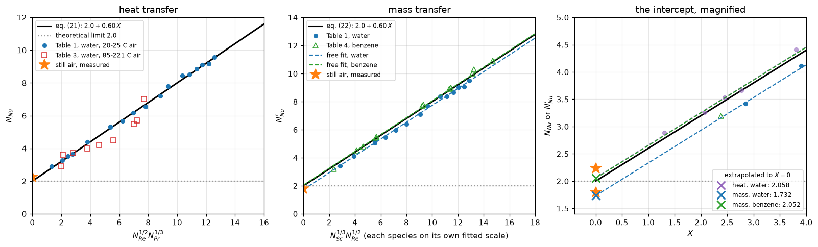
Right-hand panel: the three free two-parameter fits extrapolated to X = 0.
The stars are the paper's own still-air measurements, which are separate
experiments and are NOT in any of the three fits.
Validation
1. The theoretical 2.0, recomputed, and checked against the exact answer
Part I’s eq. (7) is asserted, not solved, and it is the only constant in the correlation worth solving for. pymrm solves the spherical BVP on a ladder of nested geometric grids, and the orders come from successive differences (pymrm.checks.observed_orders), which need no exact answer. In a shell of outer radius \(b\) the exact answer is \(2/(1-a/b)\), so the floor \(N_{Nu}(1-a/b)\) is exactly 2 at every \(b\) and only the grid needs refining. The series-resistance integral \(\int_a^\infty \mathrm{d}r/4\pi r^2 k\) is then evaluated by adaptive quadrature, sharing no grid, no assembly and no linear solve; but \(2/(4\pi\int_1^\infty
\mathrm{d}r/4\pi r^2)\) is identically 2 for any working quadrature, so it is the exact answer obtained numerically. What follows is a finite-volume solve measured against the analytic limit, not two independent estimates that happen to agree.
# WHERE THE 2.0 COMES FROM. Part I obtains it from eqs. (1), (2), (5) and (6)
# with the fluid at rest: steady conduction (or diffusion) out of a sphere into a
# stagnant medium. That is a one-dimensional spherical BVP and it is linear, so
# pymrm answers it with one sparse solve per grid: construct_div(..., nu=2) for the
# spherical geometry, on geometric faces (they nest when the cell count doubles),
# the surface gradient read with compute_boundary_values.
#
# In a shell of outer radius b the exact answer is Nu = 2/(1 - a/b), so the floor
# Nu (1 - a/b) is exactly 2 at every b: the domain size is removed in closed form
# and only the grid is refined.
RATIO = 1.0e4
NS_COND = (50, 100, 200, 400, 800, 1600)


def resistance_route(upper=np.inf):
    """The same limit as a series of shell resistances, integral of dr/(4 pi r^2 k)
    from a to the far field, by adaptive quadrature. It shares no grid, no assembly
    and no linear solve with the finite volumes; for upper = infinity it is exactly
    2 for any working quadrature, so it is the exact answer obtained numerically."""
    r_tot, _ = quad(lambda r: 1.0 / (4.0 * np.pi * r ** 2), 1.0, upper,
                    epsabs=1e-14, epsrel=1e-14)
    return 2.0 / (4.0 * np.pi * r_tot)


def conduction_study(P, ns=NS_COND, ratio=RATIO, nu=2, outer="dirichlet", geometric=True,
                     upper=np.inf):
    """The stagnant floor on a ladder of nested grids, its Richardson limit, the
    surface-against-shell flux identity, and the resistance-integral route."""
    floor = lambda n: nu_shell(n, ratio, nu=nu, outer=outer, geometric=geometric) * (1 - 1 / ratio)
    oo = observed_orders(floor, ns)
    vals = np.asarray(oo["values"])
    surf = nu_shell(ns[-1], ratio, nu=nu, outer=outer, geometric=geometric)
    shell = nu_shell(ns[-1], ratio, nu=nu, outer=outer, geometric=geometric, at="shell")
    nu_q = resistance_route(upper)
    lim = float(oo["extrapolated"])
    return {"pymrm_conduction_order_min": float(np.min(oo["orders"])),
            "pymrm_conduction_order_max": float(np.max(oo["orders"])),
            "pymrm_conduction_Nu_infinity": lim,
            "pymrm_conduction_dev_from_2": float(abs(lim - P["correlation_intercept"])),
            "pymrm_conduction_shell_gap": float(abs(surf / shell - 1)) if shell else np.inf,
            "pymrm_conduction_b10_excess_pct": float(100 * (nu_shell(ns[-1], 10.0, nu=nu, outer=outer,
                                                                     geometric=geometric) / 2 - 1)),
            "nu_quadrature_route": nu_q,
            "nu_two_routes_rel_diff": float(abs(nu_q - lim) / 2.0),
            "_finest_diff": float(abs(vals[-1] - vals[-2]) / abs(vals[-1])), "_oo": oo}


CD = conduction_study(P0)
A.update({k: v for k, v in CD.items() if not k.startswith("_")})
print(f"the floor Nu (1 - a/b) at b/a = {RATIO:.0e}, nested geometric grids:")
for n, v in zip(NS_COND, CD["_oo"]["values"]):
    print(f"  n = {n:5d}   Nu (1 - a/b) = {v:.10f}   rel {v / 2 - 1:+.3e}")
print(f"  observed orders (successive differences) "
      f"{', '.join(f'{o:.4f}' for o in CD['_oo']['orders'])}")
print(f"  Richardson limit {A['pymrm_conduction_Nu_infinity']:.10f}; from the printed "
      f"{P0['correlation_intercept']:g}: below 1e-6 (here {A['pymrm_conduction_dev_from_2']:.1e})")
print(f"  surface flux against shell flux x (b/a)^2 at {NS_COND[-1]} cells: below 1e-9 "
      f"(here {A['pymrm_conduction_shell_gap']:.1e})")
print(f"\n  quadrature of the resistance integral : Nu = {A['nu_quadrature_route']:.12f}")
print(f"  finite volumes, Richardson limit      : Nu = {A['pymrm_conduction_Nu_infinity']:.12f}")
print(f"  the two routes differ by below 1e-6 relative (here {A['nu_two_routes_rel_diff']:.1e})")
print(f"\n  a far field at ten radii: Nu = {1 + A['pymrm_conduction_b10_excess_pct']/100:.4f} x 2, "
      f"{A['pymrm_conduction_b10_excess_pct']:.1f} % above the unbounded limit")
the floor Nu (1 - a/b) at b/a = 1e+04, nested geometric grids:
n = 50 Nu (1 - a/b) = 1.9809866780 rel -9.507e-03
n = 100 Nu (1 - a/b) = 1.9954833441 rel -2.258e-03
n = 200 Nu (1 - a/b) = 1.9989040875 rel -5.480e-04
n = 400 Nu (1 - a/b) = 1.9997303942 rel -1.348e-04
n = 800 Nu (1 - a/b) = 1.9999331581 rel -3.342e-05
n = 1600 Nu (1 - a/b) = 1.9999833603 rel -8.320e-06
observed orders (successive differences) 2.0833, 2.0496, 2.0269, 2.0140
Richardson limit 1.9999998799; from the printed 2: below 1e-6 (here 1.2e-07)
surface flux against shell flux x (b/a)^2 at 1600 cells: below 1e-9 (here 5.2e-13)
quadrature of the resistance integral : Nu = 2.000000000000
finite volumes, Richardson limit : Nu = 1.999999879857
the two routes differ by below 1e-6 relative (here 6.0e-08)
a far field at ten radii: Nu = 1.1111 x 2, 11.1 % above the unbounded limitSecond order on the grid, with the orders printed above approaching 2 from above, and the Richardson limit of the ladder lies below 1e-6 from the exact 2. The flux through the outer shell, times the area ratio, matches the surface flux to the residual of the solve, which is the round-off scale every ladder difference is compared with. Every row of the break table below perturbs an input and watches a number move, which shows sensitivity and never correctness; this comparison with the exact answer is what shows correctness.
Note what the domain is for. Stopping the far field at \(b/a = 10\) and calling the answer 2.0 would be wrong by 11.1 %, and no grid refinement would reveal it; it is the failure mode a grid-convergence study is blind to.
2. Radial convection, and which average \(p_f\) is
Ranz, 1993:
“A serious limitation on extended applications, unfortunately not emphasized in the original papers, has always been crude accounting (i.e., the use of the \(D_f\) factor) for the radial convection at a spherical boundary caused by diffusion at the same boundary.”
There is no \(D_f\) in the notation of either part. The object that does that accounting is \(p_f\), and Part II’s notation (folio 180) defines it only as the “average value of \((\pi - p_A)\) across transfer path”; the identification is an inference and is labelled one here. Which average it is has a right answer, and the solver gives it.
# RANZ'S OWN CAVEAT. In 1993 he wrote that a serious limitation of the papers,
# "unfortunately not emphasized in the original papers", was the crude accounting
# for "the radial convection at a spherical boundary caused by diffusion at the
# same boundary". The object that does that accounting is p_f, defined in Part
# II's notation only as the "average value of (pi - p_A) across transfer path",
# and which average is not said.
#
# Solve the actual problem: species A diffusing out of the sphere through stagnant
# B, so the mixture itself moves radially. Diffusion by construct_grad, the radial
# convection by construct_convflux_upwind (first-order upwind), geometry by
# construct_div(nu=2), and the total molar flow W the one root of "the flow the
# solve produces equals the flow it was given" (find_roots on the physical range).
# For a fixed W the problem is linear: no Newton iteration is needed.
#
# The error has two parts: first order from the upwind convection and second order
# from the diffusion, of opposite sign. Successive-difference orders approach 1
# from below on the ladder; the two known orders are then removed together,
# q* = (8 q(h/4) - 6 q(h/2) + q(h)) / 3, and what is left falls by about 8 per
# doubling.
RS = 1.0e5
YS = (0.01, 0.05, 0.10, 0.20)
N_STEF = 600
NS_STEF = (600, 1200, 2400, 4800, 9600, 19200)


def stefan_study(ys=YS, ns=NS_STEF, y_order=0.20, convection=True):
    """Stefan flow against its closed form: the production grid, the ladder at
    y_order, the two-order Richardson limit at every y, and the balance gap."""
    prod = {y: sh_stefan(N_STEF, RS, y, convection=convection, balance=True) for y in ys}
    lad = {y: [sh_stefan(n, RS, y, convection=convection)[0] for n in ns[-3:]] for y in ys}
    oo = observed_orders(lambda n: sh_stefan(n, RS, y_order, convection=convection)[0], ns)
    ext = {y: (8 * q[2] - 6 * q[1] + q[0]) / 3 for y, q in lad.items()}
    vals = np.asarray(oo["values"])
    gap = max(p[2] for p in prod.values())
    return {"stefan_pymrm_vs_closed_rel": float(max(abs(prod[y][0] / sh_closed(RS, y) - 1)
                                                    for y in ys)),
            "stefan_order_min": float(np.min(oo["orders"])),
            "stefan_order_max": float(np.max(oo["orders"])),
            "stefan_extrap_vs_closed_rel": float(max(abs(ext[y] / sh_closed(RS, y) - 1)
                                                     for y in ys)),
            "stefan_balance_gap": float(gap),
            "_finest_diff": float(abs(vals[-1] - vals[-2]) / abs(vals[-1])),
            "_prod": prod, "_ext": ext, "_oo": oo}


ST = stefan_study()
A.update({k: v for k, v in ST.items() if not k.startswith("_")})
print(f"{'y_surface':>10}{'pymrm Sh':>14}{'closed form':>14}{'rel':>11}{'Richardson':>13}"
      f"{'rel':>11}")
for y in YS:
    s, e, x = ST["_prod"][y][0], sh_closed(RS, y), ST["_ext"][y]
    print(f"{y:10.2f}{s:14.6f}{e:14.6f}{s/e-1:11.2e}{x:13.8f}{x/e-1:11.2e}")
print(f"\n  at {N_STEF} cells the worst disagreement with the closed form is "
      f"{A['stefan_pymrm_vs_closed_rel']:.2e}")
print(f"  ladder at y = 0.20, cells {', '.join(str(n) for n in NS_STEF)}: observed orders "
      f"{', '.join(f'{o:.4f}' for o in ST['_oo']['orders'])}")
print(f"  (first-order upwind; the opposite-signed second-order diffusion error makes")
print(f"   the orders approach 1 from below)")
print(f"  the two-order Richardson limit from {NS_STEF[-3]}-{NS_STEF[-1]} cells is within "
      f"1e-8 of the closed form at every y (here {A['stefan_extrap_vs_closed_rel']:.1e})")
print(f"  flow through the outer face against the surface flow: below 1e-9 "
      f"(here {A['stefan_balance_gap']:.1e})")

# Now the question the notation leaves open. Ranz's N_Nu' carries a factor p_f/pi.
# If p_f is the LOGARITHMIC mean of (pi - p_A) it removes the radial-convection
# enhancement exactly and returns the theoretical 2.0; if it is the arithmetic
# mean it does not.
yy = np.array(YS)
sh_ext = np.array([ST["_ext"][y] for y in YS])
back_log = sh_ext * pf_log(yy) * (1 - 1 / RS)      # the pymrm limit, not the closed form
back_arith = np.array([sh_closed(RS, y) for y in YS]) * pf_arith(yy) * (1 - 1 / RS)


def pf_arith_dev(y=0.20, weight=0.5):
    """Per cent by which the closed-form Sh times the arithmetic-mean factor
    1 - weight y misses 2 at surface mole fraction y."""
    return float(100 * abs(sh_closed(RS, y) * (1 - weight * y) * (1 - 1 / RS) / 2.0 - 1))


A["pf_arith_dev_at_y020_pct"] = pf_arith_dev()
print(f"\n  pymrm Sh (Richardson) x p_f/pi, p_f the LOG mean -> "
      f"{np.array2string(back_log, precision=9)}")
print("  (with the CLOSED FORM in place of the pymrm Sh that product is exactly 2 for")
print("   every y, an algebraic identity, so it is not a claim; the line above is the")
print("   pymrm solve asked the same question, and its distance from 2 is the")
print("   Richardson-limit disagreement above, not a second number.)")
print(f"  closed-form Sh x p_f/pi, p_f the ARITHMETIC mean -> "
      f"{np.array2string(back_arith, precision=6)}")
print(f"  the arithmetic mean is {A['pf_arith_dev_at_y020_pct']:.2f} % out at y = {YS[-1]:g}.")


# How large is the effect at all? Each threshold is the one root of
# corr_excess(y) = target, and the same y has a closed form through Lambert's W.
def thresholds(targets=(0.01, 0.05, 0.10), branch=0):
    ys_ = [stefan_threshold(t_) for t_ in targets]
    lw = [stefan_threshold_lambertw(t_, branch) for t_ in targets]
    out = {f"stefan_y_for_{k}pct": y for k, y in zip(("01", "05", "10"), ys_)}
    out["stefan_threshold_vs_lambertw"] = float(max(abs(a - b) for a, b in zip(ys_, lw)))
    return out


A.update(thresholds())
for k, t_ in zip(("01", "05", "10"), (0.01, 0.05, 0.10)):
    print(f"  radial convection raises Sh by {100*t_:4.0f} % once the surface mole "
          f"fraction reaches y = {A[f'stefan_y_for_{k}pct']:.6f}")
print(f"  root against Lambert-W closed form: below 1e-12 "
      f"(here {A['stefan_threshold_vs_lambertw']:.1e})")
print("\n  Placing this paper's runs on that axis needs vapour pressures, which")
print("  Part II prints only as Figure 14, out of scope. The correction is stated")
print("  as a function of y and not evaluated at their conditions.")
y_surface pymrm Sh closed form rel Richardson rel
0.01 2.009995 2.010087 -4.58e-05 2.01008727 -3.38e-10
0.05 2.052058 2.051752 1.49e-04 2.05175229 -3.20e-10
0.10 2.108085 2.107231 4.05e-04 2.10723138 -2.90e-10
0.20 2.233605 2.231458 9.62e-04 2.23145783 -2.83e-10
at 600 cells the worst disagreement with the closed form is 9.62e-04
ladder at y = 0.20, cells 600, 1200, 2400, 4800, 9600, 19200: observed orders 0.8753, 0.9420, 0.9720, 0.9862
(first-order upwind; the opposite-signed second-order diffusion error makes
the orders approach 1 from below)
the two-order Richardson limit from 4800-19200 cells is within 1e-8 of the closed form at every y (here 3.4e-10)
flow through the outer face against the surface flow: below 1e-9 (here 2.0e-13)
pymrm Sh (Richardson) x p_f/pi, p_f the LOG mean -> [1.999999999 1.999999999 1.999999999 1.999999999]
(with the CLOSED FORM in place of the pymrm Sh that product is exactly 2 for
every y, an algebraic identity, so it is not a claim; the line above is the
pymrm solve asked the same question, and its distance from 2 is the
Richardson-limit disagreement above, not a second number.)
closed-form Sh x p_f/pi, p_f the ARITHMETIC mean -> [2.000017 2.000438 2.00185 2.008292]
the arithmetic mean is 0.41 % out at y = 0.2.
radial convection raises Sh by 1 % once the surface mole fraction reaches y = 0.019736
radial convection raises Sh by 5 % once the surface mole fraction reaches y = 0.093702
radial convection raises Sh by 10 % once the surface mole fraction reaches y = 0.176134
root against Lambert-W closed form: below 1e-12 (here 7.5e-15)
Placing this paper's runs on that axis needs vapour pressures, which
Part II prints only as Figure 14, out of scope. The correction is stated
as a function of y and not evaluated at their conditions.The logarithmic mean returns Ranz’s \(N_{Nu}'\) to 2.0 at rest: with the pymrm solution in place of the closed form, the product’s distance from 2 is the Richardson-limit disagreement, below 1e-8, and not a second number, because the log mean cancels the closed form identically. The arithmetic mean does not, and is 0.41 % out by \(y = 0.20\), far outside both the production-grid disagreement of 9.62e-4 and the limit. So \(p_f\) must be the log mean, and read that way the paper’s mass-transfer accounting for radial convection is exact, not crude, for the isothermal spherical stagnant film. What it does not do is appear anywhere in the heat balance, which is where a Stefan flow also carries enthalpy; that asymmetry is the most likely reading of the 1993 remark, and it is offered as a reading, not as a result.
The size of the effect: the radial convection lifts \(Sh\) by 1 % at a surface mole fraction of 1.97 %, 5 % at 9.37 % and 10 % at 17.61 %, each the one root of the closed-form excess on the physical range, and each matching its Lambert-W closed form. Placing this paper’s runs on that axis needs vapour pressures that exist only in Figure 14, so it is not done.
3. The paper’s own arithmetic
# PRINTED ARITHMETIC, checked and not repaired.


def printed_arithmetic(P):
    """Part I's test No. 80: 5.83 (1 - 0.028 - 0.006 - 0.011) against the printed 5.57."""
    n_app, n_cor = P["test80_Nu_apparent"], P["test80_Nu_corrected"]
    rec = n_app * (1 - P["test80_correction_sensible_heat"] - P["test80_correction_radiation"]
                   - P["test80_correction_capillary"])
    h = half_unit(KS.loc["test80_Nu_corrected", "value"])     # the printed string
    return {"test80_printed_vs_recomputed_rel": float(abs(rec - n_cor) / n_cor),
            "test80_within_printed_precision": bool(abs(rec - n_cor) <= h),
            "_test80_margin": float(abs(h - abs(rec - n_cor)) / h), "_rec": rec}


PA = printed_arithmetic(P0)
A.update({k: v for k, v in PA.items() if not k.startswith("_")})
print(f"Part I, test No. 80:  {P0['test80_Nu_apparent']:g} (1 - "
      f"{P0['test80_correction_sensible_heat']:g} - {P0['test80_correction_radiation']:g} - "
      f"{P0['test80_correction_capillary']:g}) = {PA['_rec']:.6f}")
print(f"  printed: {P0['test80_Nu_corrected']:g}.  Relative difference "
      f"{A['test80_printed_vs_recomputed_rel']:.2e}; inside half a unit of the printed last "
      f"digit: {A['test80_within_printed_precision']}.")
_c = (P0["test80_correction_sensible_heat"] + P0["test80_correction_radiation"]
      + P0["test80_correction_capillary"])
print(f"  (the three corrections together remove {100*_c:.1f} % of the apparent N_Nu, and the "
      f"largest of them, sensible heat, {100*P0['test80_correction_sensible_heat']:.1f} %.)")

# Eq. (24) against eqs. (21): consistent only for one Prandtl number.
print(f"\nPart II eq. (24) vs eqs. (21): {K_AQ:g} = {K_FIT:g} x Pr^(1/3) requires "
      f"Pr = {A['pr_air_implied_by_eq24']:.5f} for air.")
print(f"  Table 1's own {HT['_n']} rows, intercept held at {A2_:g}, give a coefficient of "
      f"{A['t1_heat_slope_at_A2']:.4f} against that {K_AQ:g}: "
      f"{100*(A['t1_heat_slope_at_A2']/K_AQ-1):+.2f} %.")
print("  This is not a second result: K_recovered = b_fixed x K/K_AQ identically, so")
print("  b_fixed/K_AQ - 1 is K_recovered/K - 1, which the heat section reported as")
print(f"  {100*(A['t1_heat_K_recovered']/K_FIT - 1):+.2f} %. It is one claim, not two.")
Part I, test No. 80: 5.83 (1 - 0.028 - 0.006 - 0.011) = 5.567650
printed: 5.57. Relative difference 4.22e-04; inside half a unit of the printed last digit: True.
(the three corrections together remove 4.5 % of the apparent N_Nu, and the largest of them, sensible heat, 2.8 %.)
Part II eq. (24) vs eqs. (21): 0.54 = 0.6 x Pr^(1/3) requires Pr = 0.72900 for air.
Table 1's own 18 rows, intercept held at 2, give a coefficient of 0.5418 against that 0.54: +0.34 %.
This is not a second result: K_recovered = b_fixed x K/K_AQ identically, so
b_fixed/K_AQ - 1 is K_recovered/K - 1, which the heat section reported as
+0.34 %. It is one claim, not two.No printed defect found. Test No. 80 recomputes to 4.2e-04 relative, inside half a unit of the printed 5.57’s last digit; and eq. (24)’s 0.54 is within 0.34 % of what Table 1’s own 18 rows give with the intercept held at 2.0. Both were checked because both could have failed; this section reports that they did not, rather than omitting a check that came out clean.
That second number is not a second result. \(K_{\rm recovered} \equiv b_{\rm fixed} \times 0.60/0.54\) identically, so “eq. (24)’s 0.54 against Table 1” and the heat section’s “\(K\) = 0.6020 against the printed 0.60” are one statement written two ways, and it is registered as one claim.
4. Claims
Every number the page states, with how it is checked. Arithmetic on the printed tables is held to FIXED; results that pass through a fit iterated to a tolerance or through a solver are held to SOLV. Orders, residuals, identities and the verdicts on the intercepts are bounds with their basis; statements over a set are exact claims with their margin.
FIXED, SOLV = 1e-6, 1e-4
CRIT = {k: float(student_t.ppf(0.975, d)) for k, d in MS["_dof"].items()}
CRIT["heat_q"] = float(student_t.ppf(0.975, HT["_dof"]))

# arithmetic on the printed tables and constants (fits by linear least squares,
# roots of exact derivatives, closed forms)
for k in ("pr_air_implied_by_eq24",
          "re_law_T_exponent_se",
          "re_law_resid_rms_pct", "re_law_resid_rms_pct_free_stream",
          "re_law_T_exponent_free_stream", "re_reference_weight_band",

          "t1_iso_Re_over_v_spread_pct",
          "t1_iso_rounding_ptp_bound_pct", "stillair_film_minus_stated_K",
          "t3_heldout_rms_pct_free_stream", "t3_heldout_rms_pct_drop_surface",
          "t3_extrapolation_K",
          "t1_heat_intercept_free", "t1_heat_intercept_se", "t1_heat_slope_free",
          "t1_heat_slope_at_A2", "t1_heat_K_recovered", "t1_heat_K_recovered_dev_pct",
          "t1_heat_eq24_rms_pct",
          "t1_heat_eq24_max_pct", "t1_heat_freefit_rms_pct", "t1_heat_null_best_rms_pct",
          "t1_mass_intercept_free", "t1_mass_intercept_se", "t1_mass_slope_free",
          "t1_mass_fit_resid_rms_pct",
          "t4_benzene_intercept_free", "t4_benzene_intercept_se", "t4_benzene_slope_free",
          "mass_intercept_dev_water_pct", "mass_intercept_dev_benzene_pct", "heat_intercept_dev_pct",
          "sc_ratio_benzene_over_water", "t4_ratio_spread_runs_10_12_pct",
          "t4_run11_Nuprime_upper_bound", "t4_run11_Nuprime_lower_bound", "t4_run11_alt_intercept",
          "t4_run11_alt_intercept_drift_pct", "t4_run11_alt_ratio_spread_pct",
          "t4_run11_alt_outside_bracket_pct",
          "stillair_Nu_over_theory", "stillair_Nuprime_over_theory", "stillair_analogy_ratio",
          "dv_used_over_dv_backed_out", "dv_factor_from_intercept", "replicate_worst_pct", "replicate_mean_pct",
          "t3_eq21_rms_pct", "t3_eq21_max_pct", "t3_eq21_bias_pct", "t3_eq21_bias_se_pct",
          "t3_from_t1_rms_pct",
          "t3_over_t1_rms_factor", "t3_pair_abscissa_max_dev_pct", "t3_pair_nu_ratio_max_dev_pct",
          "t3_pair_worst_nu_ratio_error_pct", "pf_arith_dev_at_y020_pct",
          "stefan_y_for_01pct", "stefan_y_for_05pct", "stefan_y_for_10pct",
          "test80_printed_vs_recomputed_rel"):
    claims.value(k, A[k], rtol=FIXED)
# a nonlinear least-squares fit, iterated to curve_fit's tolerance; and the values
# downstream of the reference-temperature weight w, whose measured spread across BLAS
# kernels (docs/reproducibility/spread.json) reaches 1e-7 relative
for k in ("t1_heat_Re_exponent_fitted", "t1_heat_Re_exponent_se",
          "re_reference_temperature_weight", "re_law_T_exponent", "re_law_resid_max_pct",
          "re_freestream_worst_Re_pct", "re_freestream_worst_Nu_pct",
          "t1_iso_expected_spread_from_T_pct", "t3_heldout_rms_pct", "t3_heldout_w"):
    claims.value(k, A[k], rtol=SOLV)
# the verdicts: (intercept - 2.0)/standard error, Student t under "the intercept is 2.0"
claims.bound("mass_intercept_t_water", A["mass_intercept_t_water"], max=-CRIT["water"],
             basis="chosen", note="beyond the two-sided 5 % point of Student t, 13 dof")
claims.bound("heat_intercept_t", A["heat_intercept_t"], min=-CRIT["heat"], max=CRIT["heat"],
             basis="chosen", note="inside the two-sided 5 % points of Student t, 16 dof")
claims.bound("mass_intercept_t_benzene", A["mass_intercept_t_benzene"], min=-CRIT["benzene"],
             max=CRIT["benzene"], basis="chosen",
             note="inside the two-sided 5 % points of Student t, 11 dof")
claims.bound("t1_heat_Re_exponent_t", A["t1_heat_Re_exponent_t"], min=-CRIT["heat_q"],
             max=CRIT["heat_q"], basis="chosen",
             note="released exponent against 1/2 inside the two-sided 5 % points, 16 dof")
# statements over a set
claims.exact("re_band_holds_045_and_055", A["re_band_holds_045_and_055"], margin=RE["_band_margin"],
             min_margin=0.01, note="both w = 0.45 and 0.55 inside the 5 % band; margin in w")
claims.exact("t1_iso_spread_below_T_effect", A["t1_iso_spread_below_T_effect"],
             margin=RE["_iso_margin"], min_margin=0.05,
             note="observed Re/v spread below the film-temperature effect alone; margin relative")
claims.exact("t1_iso_spread_inside_T_plus_rounding", A["t1_iso_spread_inside_T_plus_rounding"],
             margin=RE["_iso_margin2"], min_margin=0.05,
             note="observed spread inside temperature effect plus rounding; margin relative")
claims.exact("t3_pair_identities_within_rounding", A["t3_pair_identities_within_rounding"],
             margin=T3["_ident_margin"], min_margin=0.1,
             note="both within-pair identities inside their printing allowance in every pair")
STEEP = (T3["_pairs"].d / T3["_pairs"].allow_d).to_numpy()
claims.count("t3_pairs_measurement_steeper", STEEP, 0.0, min_margin=1.0, relative=False,
             note="pairs whose measured N_Nu ratio exceeds eq. (21)'s; each difference in units "
                  "of its printing allowance, margin at least one allowance")
claims.exact("test80_within_printed_precision", A["test80_within_printed_precision"],
             margin=PA["_test80_margin"], min_margin=0.05,
             note="recomputed test No. 80 within half a unit of the printed last digit")
# pymrm: the stagnant sphere
claims.value("pymrm_conduction_Nu_infinity", A["pymrm_conduction_Nu_infinity"], rtol=FIXED)
claims.value("pymrm_conduction_b10_excess_pct", A["pymrm_conduction_b10_excess_pct"], rtol=SOLV)
claims.bound("pymrm_conduction_order_min", A["pymrm_conduction_order_min"], min=1.95, basis="theory",
             note="second order on nested geometric cells")
claims.bound("pymrm_conduction_order_max", A["pymrm_conduction_order_max"], max=2.15, basis="theory",
             note="second order on nested geometric cells, approached from above")
claims.bound("pymrm_conduction_dev_from_2", A["pymrm_conduction_dev_from_2"], max=1e-6,
             basis="theory", note="Richardson limit of a second-order ladder; the next-order terms")
claims.bound("pymrm_conduction_shell_gap", A["pymrm_conduction_shell_gap"], max=1e-9,
             basis="identity", note="the discrete divergence telescopes; the gap is the solve's residual")
claims.bound("nu_quadrature_route", A["nu_quadrature_route"], min=2 - 1e-12, max=2 + 1e-12,
             basis="identity", note="2/(4 pi integral of dr/(4 pi r^2)) is 2 for any working quadrature")
claims.bound("nu_two_routes_rel_diff", A["nu_two_routes_rel_diff"], max=1e-6, basis="theory",
             note="the Richardson limit against the exact 2; the next-order terms")
# pymrm: Stefan flow
claims.value("stefan_pymrm_vs_closed_rel", A["stefan_pymrm_vs_closed_rel"], rtol=SOLV)
claims.bound("stefan_order_min", A["stefan_order_min"], min=0.85, basis="theory",
             note="first-order upwind, approached from below (second-order diffusion error of "
                  "opposite sign)")
claims.bound("stefan_order_max", A["stefan_order_max"], max=1.0, basis="theory",
             note="first-order upwind, approached from below")
claims.bound("stefan_extrap_vs_closed_rel", A["stefan_extrap_vs_closed_rel"], max=1e-8,
             basis="theory", note="orders 1 and 2 removed together; the third-order residue")
claims.bound("stefan_balance_gap", A["stefan_balance_gap"], max=1e-9, basis="identity",
             structural=True, note="r^2 times the radial flux is the same on every face of the "
                                   "discrete balance; the gap is the solve's residual")
FINEST_OVER_ROUNDOFF = (min(CD["_finest_diff"], ST["_finest_diff"])
                        / max(A["pymrm_conduction_shell_gap"], A["stefan_balance_gap"]))
claims.bound("ladder_finest_over_roundoff", FINEST_OVER_ROUNDOFF, min=1e3, basis="theory",
             note="the finest ladder differences far above the solves' residual")
claims.bound("stefan_threshold_vs_lambertw", A["stefan_threshold_vs_lambertw"], max=1e-12,
             basis="tolerance", note="root xtol 1e-15; Lambert W to round-off")
print(f"{len(claims.metrics)} claims registered")
96 claims registered5. The defect-injection table
Every claim above needs a row that fails its own check. The data claims come from analyse(D, P), the whole analysis of sections 1 to 3 as one function of the tables and the printed-constant dictionary: each row misreads one printed number (a table cell, a column, a constant) or switches one analysis choice through an argument, and reruns everything, so every claim the defect reaches is tested. The pymrm claims get rows of their own, each a call argument of the study: the geometry code, the outer condition, the grid, the ladder, the convection, the far field of the quadrature, the targets and the Lambert-W branch. A quantity that cannot be computed under a defect records nan, which fails its claim.
def public(d):
    return {k: v for k, v in d.items() if not k.startswith("_")}


def analyse(D, P, w=None, include_still=False):
    """Sections 1 to 3 rerun in full on tables D and constants P."""
    re_ = reynolds(D, P, w=w)
    out = {"pr_air_implied_by_eq24": pr_implied(P), **public(re_)}
    out.update(public(table3_heldout(D, P, re_["_w"], re_["_R"], re_["_y"])))
    ht = heat(D, P, include_still=include_still)
    ms = mass(D, P, ht)
    t3_ = table3(D, P, ht)
    out.update({**public(ht), **public(ms), **public(still_air(D, P)), **public(t3_),
                **public(printed_arithmetic(P))})
    out["t3_pairs_measurement_steeper"] = int(np.sum(t3_["_pairs"].d > 0))
    return out


BREAK = []


def brk(row, name, broken):
    """One injected defect: ``broken`` is what claim ``name`` becomes with it."""
    if isinstance(broken, (float, np.floating)) and not np.isfinite(broken):
        broken = np.nan
    BREAK.append((row, name, claims.breaks(row, name, broken)))


def data_row(label, D=D0, P=P0, **kw):
    """Rerun the analysis under one defect; register every claim it reaches."""
    try:
        a = analyse(D, P, **kw)
    except Exception as exc:                      # a defect that leaves no solution
        print(f"  {label}: no result ({type(exc).__name__}); every data claim records nan")
        a = {k: np.nan for k in A}
    for name in claims.metrics:
        if name in a:
            brk(label, name, a[name])


def with_cell(tab, run, col, val, D=None):
    """The tables with one printed cell misread, in the numbers and in the strings."""
    D = dict(D0 if D is None else D)
    D[tab], D[tab + "s"] = D[tab].copy(), D[tab + "s"].copy()
    D[tab].loc[D[tab].run == run, col] = float(val)
    D[tab + "s"].loc[D[tab + "s"].run == str(run), col] = str(val)
    return D


def with_col(tab, col, val):
    """The tables with one column misread: a value, or another column copied in."""
    D = dict(D0)
    D[tab], D[tab + "s"] = D0[tab].copy(), D0[tab + "s"].copy()
    for t in (D[tab], D[tab + "s"]):
        t[col] = val(t) if callable(val) else (val if t is D[tab] else str(val))
    return D


def with_p(key, val):
    return {**P0, key: val}


# the baseline reproduces itself (a sanity check of analyse, not a row)
_base = analyse(D0, P0)
assert all(_base[k] == A[k] for k in _base if k in A and isinstance(A[k], bool)), "analyse drifts"
assert max(abs(_base[k] / A[k] - 1) for k in _base
           if k in A and not isinstance(A[k], bool) and A[k] != 0) < 1e-12, "analyse drifts"

data_row("Table 1 run 1 N_Re read 195.1 instead of 159.1", with_cell("t1", 1, "Re", "195.1"))
data_row("Table 1 drop diameter read 0.954 instead of 0.0954 on every row",
         with_col("t1", "D_p_cm", 0.954))
data_row("Table 1 run 14 air velocity read 3.4 instead of 3.37",
         with_cell("t1", 14, "air_vel_cm_s", "3.4"))
data_row("Table 1 drop temperatures replaced by the air temperatures",
         with_col("t1", "drop_temp_C", lambda t: t.air_temp_C))
data_row("Table 1 run 6 air velocity read 92.5 instead of 95.2",
         with_cell("t1", 6, "air_vel_cm_s", "92.5"))
data_row("Table 3 drop temperatures replaced by its air temperatures",
         with_col("t3", "drop_temp_C", lambda t: t.air_temp_C))
data_row("reference temperature fixed at the free stream (w = 0)", w=0.0)
data_row("Table 1 apparent N_Nu used for the corrected column",
         with_col("t1", "Nu_corrected", lambda t: t.Nu_apparent))
data_row("still-air row swept into the heat regression", include_still=True)
data_row("Table 1 run 18 N_Nu read 6.56 instead of 9.56", with_cell("t1", 18, "Nu_corrected", "6.56"))
data_row("Table 1 run 18 N_Nu' read 4.48 instead of 9.48", with_cell("t1", 18, "Nu_prime", "4.48"))
_guess = with_cell("t1", 12, "Nu_prime", "3.32")
for run, v in ((13, "3.05"), (14, "2.96")):
    _guess = with_cell("t1", run, "Nu_prime", v, D=_guess)
data_row("the three ink-damaged N_Nu' cells filled in by guesswork", _guess)
data_row("Table 4 N_Nu' column replaced by its N_Nu column",
         with_col("t4", "Nu_prime", lambda t: t.Nu_apparent))
data_row("Table 4 run 11 N_Nu' read 10.6 instead of 10.0", with_cell("t4", 11, "Nu_prime", "10.6"))
data_row("Table 4 run 12 N_Nu' read 10.0 instead of 10.9", with_cell("t4", 12, "Nu_prime", "10.0"))
data_row("still-air N_Nu read 3.23 instead of 2.23", with_cell("t1", 19, "Nu_apparent", "3.23"))
data_row("still-air N_Nu' read 1.19 instead of 1.79", with_cell("t1", 19, "Nu_prime", "1.19"))
data_row("Table 2 run 4 corrected N_Nu read 5.9 instead of 5.4", with_cell("t2", 4, "Nu_corrected", "5.9"))
data_row("Table 3 run 7 diameter read 0.101 instead of 0.088",
         with_cell("t3", 7, "D_p_corresponding_cm", "0.101"))
data_row("Table 3 run 1 N_Nu read 4.0 instead of 7.0", with_cell("t3", 1, "Nu", "4.0"))
data_row("theoretical intercept 2.0 read as 1.7", P=with_p("correlation_intercept", 1.7))
data_row("fitted coefficient 0.60 read as 6.0", P=with_p("correlation_coefficient_K", 6.0))
data_row("Reynolds exponent 1/2 read as 1/3", P=with_p("exponent_Re", 1 / 3))
data_row("Prandtl exponent 1/3 read as 1/2", P=with_p("exponent_Pr_Sc", 0.5))
data_row("eq. (24) coefficient 0.54 read as 0.60", P=with_p("aqueous_collapsed_coefficient", 0.60))
data_row("still-air reference temperature 290 K read as 280 K", P=with_p("Dv_backout_temperature_K", 280.0))
data_row("Table 3 pressure 743 mm Hg read as 473", P=with_p("table3_pressure_mmHg", 473.0))
data_row("test No. 80 capillary correction 0.011 read as 0.001",
         P=with_p("test80_correction_capillary", 0.001))

# --- pymrm: the stagnant sphere ----------------------------------------------------------
_cd_rows = {}
for row, kw in (("sphere solved with nu = 1 (cylinder)", dict(nu=1)),
                ("sphere outer boundary closed (no flux)", dict(outer="noflux")),
                ("uniform radial cells instead of geometric", dict(geometric=False)),
                ("ladder started at 6 cells", dict(ns=(6, 12, 24, 48, 96, 192))),
                ("resistance integral stopped at 10 radii", dict(upper=10.0)),
                ("theoretical intercept 2.0 read as 1.7 in the sphere check",
                 dict(P=with_p("correlation_intercept", 1.7)))):
    kw = {"P": P0, **kw}
    _cd_rows[row] = s = conduction_study(**kw)
    for name in claims.metrics:
        if name in s:
            brk(row, name, s[name])
_s1 = _cd_rows["sphere solved with nu = 1 (cylinder)"]
brk("sphere solved with nu = 1 (cylinder)", "ladder_finest_over_roundoff",
    min(_s1["_finest_diff"], ST["_finest_diff"])
    / max(_s1["pymrm_conduction_shell_gap"], A["stefan_balance_gap"]))

# --- pymrm: Stefan flow --------------------------------------------------------------------
for row, kw in (("radial convection switched off in the Stefan solve", dict(convection=False)),
                ("Stefan order ladder run at y = 0.01", dict(y_order=0.01))):
    s = stefan_study(**kw)
    for name in ("stefan_pymrm_vs_closed_rel", "stefan_order_min", "stefan_order_max",
                 "stefan_extrap_vs_closed_rel"):
        brk(row, name, s[name])
brk("p_f arithmetic mean taken as 1 - y", "pf_arith_dev_at_y020_pct", pf_arith_dev(weight=1.0))
_th = thresholds(targets=(0.02, 0.07, 0.15))
for k in ("01", "05", "10"):
    brk("thresholds solved for 2, 7 and 15 % instead of 1, 5 and 10 %", f"stefan_y_for_{k}pct",
        _th[f"stefan_y_for_{k}pct"])
brk("Lambert W on the branch W_-1", "stefan_threshold_vs_lambertw",
    thresholds(branch=-1)["stefan_threshold_vs_lambertw"])

bt = pd.DataFrame(BREAK, columns=["row", "claim", "caught"])
caught = bt[bt.caught].groupby("row", sort=False).claim.apply(list)
print(f"{len(bt.row.unique())} rows; claims each row fails:")
for row, names in caught.items():
    print(f"  {row}: {len(names)}")
    print("      " + ", ".join(names))
idle = [r for r in bt.row.unique() if r not in caught.index]
print(f"\nrows that fail no claim: {idle if idle else 'none'}")
missing = [n for n in claims.metrics
           if not claims.metrics[n].get("structural") and not bt[(bt.claim == n) & bt.caught].shape[0]]
print(f"claims no row fails: {missing if missing else 'none'}")
39 rows; claims each row fails:
Table 1 run 1 N_Re read 195.1 instead of 159.1: 41
re_law_T_exponent_se, re_law_resid_rms_pct, re_law_resid_rms_pct_free_stream, re_law_T_exponent_free_stream, re_reference_weight_band, t3_heldout_rms_pct_free_stream, t3_heldout_rms_pct_drop_surface, t3_extrapolation_K, t1_heat_intercept_free, t1_heat_intercept_se, t1_heat_slope_free, t1_heat_slope_at_A2, t1_heat_K_recovered, t1_heat_K_recovered_dev_pct, t1_heat_eq24_rms_pct, t1_heat_eq24_max_pct, t1_heat_freefit_rms_pct, t1_heat_null_best_rms_pct, t1_mass_intercept_free, t1_mass_intercept_se, t1_mass_slope_free, t1_mass_fit_resid_rms_pct, mass_intercept_dev_water_pct, heat_intercept_dev_pct, sc_ratio_benzene_over_water, dv_factor_from_intercept, t3_from_t1_rms_pct, t3_over_t1_rms_factor, t1_heat_Re_exponent_fitted, t1_heat_Re_exponent_se, re_reference_temperature_weight, re_law_T_exponent, re_law_resid_max_pct, re_freestream_worst_Re_pct, re_freestream_worst_Nu_pct, t1_iso_expected_spread_from_T_pct, t3_heldout_rms_pct, t3_heldout_w, mass_intercept_t_water, re_band_holds_045_and_055, t1_iso_spread_below_T_effect
Table 1 drop diameter read 0.954 instead of 0.0954 on every row: 19
re_law_T_exponent_se, re_law_resid_rms_pct, re_law_resid_rms_pct_free_stream, re_law_T_exponent_free_stream, re_reference_weight_band, t3_heldout_rms_pct_free_stream, t3_heldout_rms_pct_drop_surface, t3_extrapolation_K, re_reference_temperature_weight, re_law_T_exponent, re_law_resid_max_pct, re_freestream_worst_Re_pct, re_freestream_worst_Nu_pct, t1_iso_expected_spread_from_T_pct, t3_heldout_rms_pct, t3_heldout_w, re_band_holds_045_and_055, t1_iso_spread_below_T_effect, t1_iso_spread_inside_T_plus_rounding
Table 1 run 14 air velocity read 3.4 instead of 3.37: 19
re_law_T_exponent_se, re_law_resid_rms_pct, re_law_resid_rms_pct_free_stream, re_law_T_exponent_free_stream, re_reference_weight_band, t1_iso_Re_over_v_spread_pct, t1_iso_rounding_ptp_bound_pct, t3_heldout_rms_pct_free_stream, t3_heldout_rms_pct_drop_surface, t3_extrapolation_K, re_reference_temperature_weight, re_law_T_exponent, re_law_resid_max_pct, re_freestream_worst_Re_pct, re_freestream_worst_Nu_pct, t1_iso_expected_spread_from_T_pct, t3_heldout_rms_pct, t3_heldout_w, t1_iso_spread_below_T_effect
Table 1 drop temperatures replaced by the air temperatures: 16
re_law_T_exponent_se, re_law_resid_rms_pct, re_reference_weight_band, stillair_film_minus_stated_K, t3_heldout_rms_pct_drop_surface, t3_extrapolation_K, re_reference_temperature_weight, re_law_T_exponent, re_law_resid_max_pct, re_freestream_worst_Re_pct, re_freestream_worst_Nu_pct, t1_iso_expected_spread_from_T_pct, t3_heldout_rms_pct, t3_heldout_w, re_band_holds_045_and_055, t1_iso_spread_below_T_effect
Table 1 run 6 air velocity read 92.5 instead of 95.2: 19
re_law_T_exponent_se, re_law_resid_rms_pct, re_law_resid_rms_pct_free_stream, re_law_T_exponent_free_stream, re_reference_weight_band, t1_iso_Re_over_v_spread_pct, t3_heldout_rms_pct_free_stream, t3_heldout_rms_pct_drop_surface, t3_extrapolation_K, re_reference_temperature_weight, re_law_T_exponent, re_law_resid_max_pct, re_freestream_worst_Re_pct, re_freestream_worst_Nu_pct, t1_iso_expected_spread_from_T_pct, t3_heldout_rms_pct, t3_heldout_w, t1_iso_spread_below_T_effect, t1_iso_spread_inside_T_plus_rounding
Table 3 drop temperatures replaced by its air temperatures: 4
t3_heldout_rms_pct_drop_surface, t3_extrapolation_K, t3_heldout_rms_pct, t3_heldout_w
reference temperature fixed at the free stream (w = 0): 13
re_law_T_exponent_se, re_law_resid_rms_pct, re_reference_weight_band, t3_extrapolation_K, re_reference_temperature_weight, re_law_T_exponent, re_law_resid_max_pct, re_freestream_worst_Re_pct, re_freestream_worst_Nu_pct, t1_iso_expected_spread_from_T_pct, t3_heldout_rms_pct, re_band_holds_045_and_055, t1_iso_spread_below_T_effect
Table 1 apparent N_Nu used for the corrected column: 17
t1_heat_intercept_free, t1_heat_intercept_se, t1_heat_slope_free, t1_heat_slope_at_A2, t1_heat_K_recovered, t1_heat_K_recovered_dev_pct, t1_heat_eq24_rms_pct, t1_heat_eq24_max_pct, t1_heat_freefit_rms_pct, t1_heat_null_best_rms_pct, heat_intercept_dev_pct, replicate_mean_pct, t3_from_t1_rms_pct, t3_over_t1_rms_factor, t1_heat_Re_exponent_fitted, t1_heat_Re_exponent_se, heat_intercept_t
still-air row swept into the heat regression: 10
t1_heat_intercept_free, t1_heat_intercept_se, t1_heat_slope_free, t1_heat_eq24_rms_pct, t1_heat_eq24_max_pct, t1_heat_freefit_rms_pct, t1_heat_null_best_rms_pct, heat_intercept_dev_pct, t3_over_t1_rms_factor, t1_heat_Re_exponent_se
Table 1 run 18 N_Nu read 6.56 instead of 9.56: 15
t1_heat_intercept_free, t1_heat_intercept_se, t1_heat_slope_free, t1_heat_slope_at_A2, t1_heat_K_recovered, t1_heat_K_recovered_dev_pct, t1_heat_eq24_rms_pct, t1_heat_eq24_max_pct, t1_heat_freefit_rms_pct, t1_heat_null_best_rms_pct, heat_intercept_dev_pct, t3_from_t1_rms_pct, t3_over_t1_rms_factor, t1_heat_Re_exponent_fitted, t1_heat_Re_exponent_se
Table 1 run 18 N_Nu' read 4.48 instead of 9.48: 8
t1_mass_intercept_free, t1_mass_intercept_se, t1_mass_slope_free, t1_mass_fit_resid_rms_pct, mass_intercept_dev_water_pct, sc_ratio_benzene_over_water, dv_factor_from_intercept, mass_intercept_t_water
the three ink-damaged N_Nu' cells filled in by guesswork: 8
t1_mass_intercept_free, t1_mass_intercept_se, t1_mass_slope_free, t1_mass_fit_resid_rms_pct, mass_intercept_dev_water_pct, sc_ratio_benzene_over_water, dv_factor_from_intercept, mass_intercept_t_water
Table 4 N_Nu' column replaced by its N_Nu column: 13
t4_benzene_intercept_free, t4_benzene_intercept_se, t4_benzene_slope_free, mass_intercept_dev_benzene_pct, sc_ratio_benzene_over_water, t4_ratio_spread_runs_10_12_pct, t4_run11_Nuprime_upper_bound, t4_run11_Nuprime_lower_bound, t4_run11_alt_intercept, t4_run11_alt_intercept_drift_pct, t4_run11_alt_ratio_spread_pct, t4_run11_alt_outside_bracket_pct, mass_intercept_t_benzene
Table 4 run 11 N_Nu' read 10.6 instead of 10.0: 7
t4_benzene_intercept_free, t4_benzene_intercept_se, t4_benzene_slope_free, mass_intercept_dev_benzene_pct, sc_ratio_benzene_over_water, t4_ratio_spread_runs_10_12_pct, t4_run11_alt_intercept_drift_pct
Table 4 run 12 N_Nu' read 10.0 instead of 10.9: 12
t4_benzene_intercept_free, t4_benzene_intercept_se, t4_benzene_slope_free, mass_intercept_dev_benzene_pct, sc_ratio_benzene_over_water, t4_ratio_spread_runs_10_12_pct, t4_run11_Nuprime_upper_bound, t4_run11_Nuprime_lower_bound, t4_run11_alt_intercept, t4_run11_alt_intercept_drift_pct, t4_run11_alt_ratio_spread_pct, t4_run11_alt_outside_bracket_pct
still-air N_Nu read 3.23 instead of 2.23: 2
stillair_Nu_over_theory, stillair_analogy_ratio
still-air N_Nu' read 1.19 instead of 1.79: 3
stillair_Nuprime_over_theory, stillair_analogy_ratio, dv_used_over_dv_backed_out
Table 2 run 4 corrected N_Nu read 5.9 instead of 5.4: 2
replicate_worst_pct, replicate_mean_pct
Table 3 run 7 diameter read 0.101 instead of 0.088: 6
t3_heldout_rms_pct_free_stream, t3_heldout_rms_pct_drop_surface, t3_pair_abscissa_max_dev_pct, t3_heldout_rms_pct, t3_heldout_w, t3_pair_identities_within_rounding
Table 3 run 1 N_Nu read 4.0 instead of 7.0: 10
t3_eq21_rms_pct, t3_eq21_max_pct, t3_eq21_bias_pct, t3_eq21_bias_se_pct, t3_from_t1_rms_pct, t3_over_t1_rms_factor, t3_pair_nu_ratio_max_dev_pct, t3_pair_worst_nu_ratio_error_pct, t3_pair_identities_within_rounding, t3_pairs_measurement_steeper
theoretical intercept 2.0 read as 1.7: 27
t1_heat_slope_at_A2, t1_heat_K_recovered, t1_heat_K_recovered_dev_pct, t1_heat_eq24_rms_pct, t1_heat_eq24_max_pct, mass_intercept_dev_water_pct, mass_intercept_dev_benzene_pct, heat_intercept_dev_pct, sc_ratio_benzene_over_water, stillair_Nu_over_theory, stillair_Nuprime_over_theory, dv_used_over_dv_backed_out, dv_factor_from_intercept, t3_eq21_rms_pct, t3_eq21_max_pct, t3_eq21_bias_pct, t3_eq21_bias_se_pct, t3_from_t1_rms_pct, t3_over_t1_rms_factor, t3_pair_worst_nu_ratio_error_pct, t1_heat_Re_exponent_fitted, t1_heat_Re_exponent_se, re_freestream_worst_Nu_pct, mass_intercept_t_water, heat_intercept_t, mass_intercept_t_benzene, t1_heat_Re_exponent_t
fitted coefficient 0.60 read as 6.0: 14
pr_air_implied_by_eq24, t3_heldout_rms_pct_free_stream, t3_heldout_rms_pct_drop_surface, t1_heat_K_recovered, t3_eq21_rms_pct, t3_eq21_max_pct, t3_eq21_bias_pct, t3_eq21_bias_se_pct, t3_from_t1_rms_pct, t3_over_t1_rms_factor, t3_pair_worst_nu_ratio_error_pct, t3_heldout_rms_pct, t3_heldout_w, t3_pairs_measurement_steeper
Reynolds exponent 1/2 read as 1/3: 34
t3_heldout_rms_pct_free_stream, t3_heldout_rms_pct_drop_surface, t1_heat_intercept_free, t1_heat_intercept_se, t1_heat_slope_free, t1_heat_slope_at_A2, t1_heat_K_recovered, t1_heat_K_recovered_dev_pct, t1_heat_eq24_rms_pct, t1_heat_eq24_max_pct, t1_heat_freefit_rms_pct, t1_heat_null_best_rms_pct, t1_mass_intercept_free, t1_mass_intercept_se, t1_mass_slope_free, t1_mass_fit_resid_rms_pct, t4_benzene_intercept_free, t4_benzene_intercept_se, t4_benzene_slope_free, mass_intercept_dev_water_pct, mass_intercept_dev_benzene_pct, heat_intercept_dev_pct, sc_ratio_benzene_over_water, t4_run11_alt_intercept, t4_run11_alt_intercept_drift_pct, dv_factor_from_intercept, t3_from_t1_rms_pct, t3_over_t1_rms_factor, re_freestream_worst_Nu_pct, t3_heldout_rms_pct, t3_heldout_w, heat_intercept_t, mass_intercept_t_benzene, t1_heat_Re_exponent_t
Prandtl exponent 1/3 read as 1/2: 2
pr_air_implied_by_eq24, sc_ratio_benzene_over_water
eq. (24) coefficient 0.54 read as 0.60: 13
pr_air_implied_by_eq24, t3_heldout_rms_pct_free_stream, t3_heldout_rms_pct_drop_surface, t1_heat_K_recovered, t1_heat_K_recovered_dev_pct, t1_heat_eq24_rms_pct, t1_heat_eq24_max_pct, t1_heat_null_best_rms_pct, t3_from_t1_rms_pct, t3_over_t1_rms_factor, re_freestream_worst_Nu_pct, t3_heldout_rms_pct, t3_heldout_w
still-air reference temperature 290 K read as 280 K: 1
stillair_film_minus_stated_K
Table 3 pressure 743 mm Hg read as 473: 4
t3_heldout_rms_pct_free_stream, t3_heldout_rms_pct_drop_surface, t3_heldout_rms_pct, t3_heldout_w
test No. 80 capillary correction 0.011 read as 0.001: 2
test80_printed_vs_recomputed_rel, test80_within_printed_precision
sphere solved with nu = 1 (cylinder): 6
pymrm_conduction_Nu_infinity, pymrm_conduction_b10_excess_pct, pymrm_conduction_dev_from_2, pymrm_conduction_shell_gap, nu_two_routes_rel_diff, ladder_finest_over_roundoff
sphere outer boundary closed (no flux): 7
pymrm_conduction_Nu_infinity, pymrm_conduction_b10_excess_pct, pymrm_conduction_order_min, pymrm_conduction_order_max, pymrm_conduction_dev_from_2, pymrm_conduction_shell_gap, nu_two_routes_rel_diff
uniform radial cells instead of geometric: 4
pymrm_conduction_Nu_infinity, pymrm_conduction_order_min, pymrm_conduction_dev_from_2, nu_two_routes_rel_diff
ladder started at 6 cells: 5
pymrm_conduction_Nu_infinity, pymrm_conduction_b10_excess_pct, pymrm_conduction_order_min, pymrm_conduction_dev_from_2, nu_two_routes_rel_diff
resistance integral stopped at 10 radii: 2
nu_quadrature_route, nu_two_routes_rel_diff
theoretical intercept 2.0 read as 1.7 in the sphere check: 1
pymrm_conduction_dev_from_2
radial convection switched off in the Stefan solve: 3
stefan_pymrm_vs_closed_rel, stefan_order_max, stefan_extrap_vs_closed_rel
Stefan order ladder run at y = 0.01: 2
stefan_order_min, stefan_order_max
p_f arithmetic mean taken as 1 - y: 1
pf_arith_dev_at_y020_pct
thresholds solved for 2, 7 and 15 % instead of 1, 5 and 10 %: 3
stefan_y_for_01pct, stefan_y_for_05pct, stefan_y_for_10pct
Lambert W on the branch W_-1: 1
stefan_threshold_vs_lambertw
rows that fail no claim: none
claims no row fails: noneWhat the break table cannot do. Every row perturbs an input and watches a claim fail. That establishes sensitivity. It cannot catch a baseline that is wrong by accident: a value limited by a grid, read at the wrong place, or right for the wrong reason. Four defences are used instead: the finite-volume 2.0 is measured against the exact answer, not against a second estimate; every threshold and minimum is a root (of the closed-form excess, of the exact derivative of the residual), not a sampled value; the datasets are checked against over-determinations the papers cannot avoid (the Reynolds column against the columns beside it, and Table 4’s \(N_{Nu}'/N_{Nu}\) ratio against its own temperature columns); and the recovered reference temperature is checked out of sample, on Table 3’s nine rows, and against the one place the papers state the convention themselves.
A constraint, not a perturbation, decides Table 4’s run 11. Read as 10.6, the digit moves the benzene intercept by only 1.5 %, inside any 5 % regression tolerance. What excludes it is the row’s \(N_{Nu}'/N_{Nu}\) ratio, which must match its neighbours’ and would not, 6.93 % against 1.03 %. A break table tells you which numbers are load-bearing; only a constraint tells you whether one is wrong.
What pymrm adds
Not the correlation. Eqs. (21) and (22) are algebra and need no solver; this page says so rather than dressing an evaluation up as a simulation. Two things are pymrm’s, and two need no solver at all.
The
2.0becomes a computation instead of a citation. Part I asserts eq. (7); pymrm solves the spherical BVP it comes from, a linear problem with one sparse solve per grid, on a ladder of nested grids whose second-order Richardson limit lies below 1e-6 from the exact 2. That matters practically, not decoratively: the same solve says a finite far field of ten radii shifts the “2” by 11.1 %, which is the correction anyone applying Ranz-Marshall inside a dense spray or a packed bed needs and which the correlation itself cannot express. (A3.4, Wakao-Funazkri, is the page for packed beds; this one does not go there.)A number on the radial-convection factor Ranz said the papers underplayed. Adding
construct_convflux_upwindto the same spherical solve, with the total flow a root of the flux balance, turns “which average is \(p_f\)?”, a genuine ambiguity in Part II’s own notation, into a settled question: the logarithmic mean, to below 1e-8 once the first-order upwind error and the second-order diffusion error are removed together; the arithmetic mean is 0.41 % out at \(y = 0.20\).The fit/test split, which is the actual result and needed no solver. Separating the theoretical 2.0 from the fitted 0.60 and the assumed exponents, and then extrapolating three independent sets of runs to \(N_{Re}=0\) with the intercept’s standard error, is what turns “the correlation fits the data to a few per cent” into “two of the three are consistent with 2.0 and the third misses by -13.4 %, 3.08 standard errors, in the direction the authors’ own first-listed error term predicts”. The authors state the direction (“Data for mass transfer show a steeper slope and a lower intercept”) and name the cause (“(1) inaccurate values of diffusivity”). What is new here is the size, per species, with its standard error, and the resulting tension with the two conclusions they did draw from it: the abstract’s “verified the simple expression for the Nusselt number at zero Reynolds number”, and folio 174’s implication that their \(D_v\) “may be more accurate than any reported in the literature”.
A convention recovered from the tables, and then tested out of sample, with no solver. The Reynolds column is over-determined by the columns printed beside it; asking it at what temperature the air properties were evaluated returns \(w\) = 0.4996, the film temperature. Two things then corroborate it independently: Part II’s own statement of a reference temperature for the still-air run (0.15 K from the row’s film temperature), and Table 3, nine rows with no Reynolds column, which therefore cannot have entered the fit, predicted to 0.82 % against 1.77 % at the free stream.
Reuse
Use Nu = 2 + 0.6 Re^(1/2) Pr^(1/3) for an isolated sphere or drop in a moving fluid at 0 < Re < 200. That is what the paper’s own abstract claims (“a Reynolds number range of 0 to 200”), and it covers Tables 1–3; note that Table 4’s last benzene run is printed at \(N_{Re} = 220\), so the tables reach slightly past the stated range. Part I’s abstract, not Part II, says the results “could be extrapolated with remarkable accuracy five times beyond the experimental range of Reynolds numbers”; Part II puts it as “remarkably accurate even when extrapolated five times beyond the experimental range in which they were determined” (folio 174). Either way that claim rests on Figure 12, which is not transcribed here, so this page neither supports nor contradicts it.
Five warnings, all of them measured above.
- Evaluate the air properties at the film temperature, the mean of the air and drop temperatures. Neither part states this for the tables; it is recovered on this page from the printed Reynolds column, at \(w\) = 0.4996 with the fitted temperature exponent landing on kinetic theory’s \(-1.7\), and it is corroborated both by the one reference temperature Part II does print (0.15 K from the row’s film temperature) and out of sample on Table 3. Using the free-stream temperature instead moves \(N_{Re}\) by up to 15.5 % on the paper’s own rows and the predicted \(N_{Nu}\) by up to 5.4 %.
- The Prandtl exponent is not testable from anything transcribed here, but the paper does test it, graphically. Every run in Tables 1–4 is in air, so the \(1/3\) cannot be identified from these rows. Figure 12 carries Kramers’s steel-to-oil and steel-to-water points on the \(N_{Pr}^{1/3}N_{Re}^{1/2}\) abscissa and folio 174 credits the exponents on that basis. That figure is not digitised here, so if your fluid is not air the \(1/3\) reaches you supported by a plot this page did not check, not by nothing; and the coefficient and the exponent are still not separable from these tables.
- Expect roughly 10 % at high air temperature. Table 3 (85–221 °C) sits 11.0 % rms from the correlation while inside its own fit set, against 1.72 % for the room-temperature runs.
- The heat and mass forms are not interchangeable at low Reynolds number. The paper’s own still-air pair has a ratio of 1.2458 where the two equations demand identity.
- If you use the mass-transfer form, watch which diffusivity you pair it with. \(N_{Nu}'\) was reduced from rate data using the authors’ own \(D_v\); adopting a different one rescales the whole correlation. A diffusivity 1.155 times too large would produce the -13.4 % intercept deficit found here; the page measures that size, not that this is its cause. The authors list “inaccurate values of diffusivity” first among the causes of the anomaly themselves, and separately conclude that their \(D_v\) may be the most accurate available; those two statements pull in opposite directions and this page cannot settle which is right.
Do not use this page for: free convection (the \(N_{Gr}^{1/4}\) form of eqs. 10 and 11 is never exercised here; say so if you cite it); drops containing dissolved or suspended solids (Part II’s second half, whose calculated rates need Figure 14); or packed beds, which is A3.4.
Datasets are reusable on their own. All five carry columns: blocks and provenance sidecars, and all five are table transcriptions, so nothing in them depends on a figure reading or on this page’s argument.
6. Prose numbers
Every number the Markdown above writes from a computed value, checked against its claim to one unit in its last written place.
PROSE = [
    ("2.0582", "t1_heat_intercept_free"), ("0.0538", "t1_heat_intercept_se"),
    ("+2.9", "heat_intercept_dev_pct"), ("1.1", "heat_intercept_t"),
    ("2.0523", "t4_benzene_intercept_free"), ("0.1245", "t4_benzene_intercept_se"),
    ("+2.6", "mass_intercept_dev_benzene_pct"), ("0.4", "mass_intercept_t_benzene"),
    ("1.7322", "t1_mass_intercept_free"), ("0.0870", "t1_mass_intercept_se"),
    ("-13.4", "mass_intercept_dev_water_pct"), ("-3.1", "mass_intercept_t_water"),
    ("1.2458", "stillair_analogy_ratio"), ("1.117", "dv_used_over_dv_backed_out"),
    ("below 1e-6", "pymrm_conduction_dev_from_2"),
    ("0.4996", "re_reference_temperature_weight"), ("-1.765", "re_law_T_exponent"),
    ("0.027", "re_law_T_exponent_se"), ("0.69", "re_law_resid_rms_pct"),
    ("-1.32", "re_law_T_exponent_free_stream"),
    ("1.14", "re_law_resid_rms_pct_free_stream"), ("0.15", "stillair_film_minus_stated_K"),
    ("15.5", "re_freestream_worst_Re_pct"), ("5.4", "re_freestream_worst_Nu_pct"),
    ("0.178", "re_reference_weight_band"), ("0.578", "t1_iso_expected_spread_from_T_pct"),
    ("0.492", "t1_iso_Re_over_v_spread_pct"), ("0.612", "t1_iso_rounding_ptp_bound_pct"),
    ("0.82", "t3_heldout_rms_pct"), ("1.77", "t3_heldout_rms_pct_free_stream"),
    ("7.20", "t3_heldout_rms_pct_drop_surface"), ("0.5140", "t3_heldout_w"),
    ("81", "t3_extrapolation_K"), ("0.729", "pr_air_implied_by_eq24"),
    ("0.6020", "t1_heat_K_recovered"), ("0.4933", "t1_heat_Re_exponent_fitted"),
    ("0.0079", "t1_heat_Re_exponent_se"), ("-0.84", "t1_heat_Re_exponent_t"),
    ("1.72", "t1_heat_eq24_rms_pct"), ("39.8", "t1_heat_null_best_rms_pct"),
    ("+1.08", "heat_intercept_t"), ("+0.42", "mass_intercept_t_benzene"),
    ("-3.08", "mass_intercept_t_water"), ("9.73", "t4_run11_Nuprime_lower_bound"),
    ("10.06", "t4_run11_Nuprime_upper_bound"), ("1.03", "t4_ratio_spread_runs_10_12_pct"),
    ("2.0222", "t4_run11_alt_intercept"), ("1.5", "t4_run11_alt_intercept_drift_pct"),
    ("6.93", "t4_run11_alt_ratio_spread_pct"), ("2.82", "sc_ratio_benzene_over_water"),
    ("0.68", "replicate_mean_pct"), ("1.87", "replicate_worst_pct"),
    ("1.155", "dv_factor_from_intercept"), ("1.44", "t1_mass_fit_resid_rms_pct"),
    ("11.0", "t3_eq21_rms_pct"), ("19.1", "t3_eq21_max_pct"), ("+6.4", "t3_eq21_bias_pct"),
    ("3.2", "t3_eq21_bias_se_pct"), ("6.4", "t3_over_t1_rms_factor"),
    ("11.2", "t3_from_t1_rms_pct"), ("1.78", "t3_pair_abscissa_max_dev_pct"),
    ("1.82", "t3_pair_nu_ratio_max_dev_pct"), ("21.9", "t3_pair_worst_nu_ratio_error_pct"),
    ("3", "t3_pairs_measurement_steeper"), ("11.1", "pymrm_conduction_b10_excess_pct"),
    ("below 1e-8", "stefan_extrap_vs_closed_rel"), ("0.41", "pf_arith_dev_at_y020_pct"),
    ("9.62e-4", "stefan_pymrm_vs_closed_rel"), ("1.97 %", "stefan_y_for_01pct"),
    ("9.37 %", "stefan_y_for_05pct"), ("17.61 %", "stefan_y_for_10pct"),
    ("4.2e-04", "test80_printed_vs_recomputed_rel"),
    ("+0.34", "t1_heat_K_recovered_dev_pct"), ("0.34", "t1_heat_K_recovered_dev_pct"),
]
bad = [(lit, name) for lit, name in PROSE if not claims.says(lit, name)]
print(f"{len(PROSE)} prose numbers checked; failing: {bad if bad else 'none'}")
74 prose numbers checked; failing: none# Claims: prints every registered number, writes agreement.json for CI, and
# raises if any claim fails its check or has no break row that fails it.
claims.report(); # the semicolon keeps the notebook from echoing the payloadClaims for A3.5:
pr_air_implied_by_eq24 = 0.729 value rtol 1e-06
re_law_T_exponent_se = 0.026515 value rtol 1e-06
re_law_resid_rms_pct = 0.69464 value rtol 1e-06
re_law_resid_rms_pct_free_stream = 1.1413 value rtol 1e-06
re_law_T_exponent_free_stream = -1.3227 value rtol 1e-06
re_reference_weight_band = 0.1778 value rtol 1e-06
t1_iso_Re_over_v_spread_pct = 0.49195 value rtol 1e-06
t1_iso_rounding_ptp_bound_pct = 0.61218 value rtol 1e-06
stillair_film_minus_stated_K = 0.15 value rtol 1e-06
t3_heldout_rms_pct_free_stream = 1.7686 value rtol 1e-06
t3_heldout_rms_pct_drop_surface = 7.2012 value rtol 1e-06
t3_extrapolation_K = 80.647 value rtol 1e-06
t1_heat_intercept_free = 2.0582 value rtol 1e-06
t1_heat_intercept_se = 0.053788 value rtol 1e-06
t1_heat_slope_free = 0.53611 value rtol 1e-06
t1_heat_slope_at_A2 = 0.54183 value rtol 1e-06
t1_heat_K_recovered = 0.60203 value rtol 1e-06
t1_heat_K_recovered_dev_pct = 0.33848 value rtol 1e-06
t1_heat_eq24_rms_pct = 1.7157 value rtol 1e-06
t1_heat_eq24_max_pct = 3.6541 value rtol 1e-06
t1_heat_freefit_rms_pct = 1.4574 value rtol 1e-06
t1_heat_null_best_rms_pct = 39.806 value rtol 1e-06
t1_mass_intercept_free = 1.7322 value rtol 1e-06
t1_mass_intercept_se = 0.087011 value rtol 1e-06
t1_mass_slope_free = 0.55396 value rtol 1e-06
t1_mass_fit_resid_rms_pct = 1.4413 value rtol 1e-06
t4_benzene_intercept_free = 2.0523 value rtol 1e-06
t4_benzene_intercept_se = 0.1245 value rtol 1e-06
t4_benzene_slope_free = 0.74106 value rtol 1e-06
mass_intercept_dev_water_pct = -13.389 value rtol 1e-06
mass_intercept_dev_benzene_pct = 2.6141 value rtol 1e-06
heat_intercept_dev_pct = 2.9122 value rtol 1e-06
sc_ratio_benzene_over_water = 2.8178 value rtol 1e-06
t4_ratio_spread_runs_10_12_pct = 1.0298 value rtol 1e-06
t4_run11_Nuprime_upper_bound = 10.064 value rtol 1e-06
t4_run11_Nuprime_lower_bound = 9.734 value rtol 1e-06
t4_run11_alt_intercept = 2.0222 value rtol 1e-06
t4_run11_alt_intercept_drift_pct = 1.4671 value rtol 1e-06
t4_run11_alt_ratio_spread_pct = 6.9305 value rtol 1e-06
t4_run11_alt_outside_bracket_pct = 5.9939 value rtol 1e-06
stillair_Nu_over_theory = 1.115 value rtol 1e-06
stillair_Nuprime_over_theory = 0.895 value rtol 1e-06
stillair_analogy_ratio = 1.2458 value rtol 1e-06
dv_used_over_dv_backed_out = 1.1173 value rtol 1e-06
dv_factor_from_intercept = 1.1546 value rtol 1e-06
replicate_worst_pct = 1.8692 value rtol 1e-06
replicate_mean_pct = 0.68129 value rtol 1e-06
t3_eq21_rms_pct = 11.047 value rtol 1e-06
t3_eq21_max_pct = 19.111 value rtol 1e-06
t3_eq21_bias_pct = 6.4422 value rtol 1e-06
t3_eq21_bias_se_pct = 3.1727 value rtol 1e-06
t3_from_t1_rms_pct = 11.191 value rtol 1e-06
t3_over_t1_rms_factor = 6.4387 value rtol 1e-06
t3_pair_abscissa_max_dev_pct = 1.7815 value rtol 1e-06
t3_pair_nu_ratio_max_dev_pct = 1.8182 value rtol 1e-06
t3_pair_worst_nu_ratio_error_pct = 21.853 value rtol 1e-06
pf_arith_dev_at_y020_pct = 0.4146 value rtol 1e-06
stefan_y_for_01pct = 0.019736 value rtol 1e-06
stefan_y_for_05pct = 0.093702 value rtol 1e-06
stefan_y_for_10pct = 0.17613 value rtol 1e-06
test80_printed_vs_recomputed_rel = 0.0004219 value rtol 1e-06
t1_heat_Re_exponent_fitted = 0.49334 value rtol 0.0001
t1_heat_Re_exponent_se = 0.0078891 value rtol 0.0001
re_reference_temperature_weight = 0.49958 value rtol 0.0001
re_law_T_exponent = -1.765 value rtol 0.0001
re_law_resid_max_pct = 2.4624 value rtol 0.0001
re_freestream_worst_Re_pct = 15.547 value rtol 0.0001
re_freestream_worst_Nu_pct = 5.4138 value rtol 0.0001
t1_iso_expected_spread_from_T_pct = 0.57849 value rtol 0.0001
t3_heldout_rms_pct = 0.82281 value rtol 0.0001
t3_heldout_w = 0.51399 value rtol 0.0001
mass_intercept_t_water = (here -3.1e+00) bound bound <= -2.16037 [chosen]
heat_intercept_t = (here 1.1e+00) bound bound [-2.11991, 2.11991] [chosen]
mass_intercept_t_benzene = (here 4.2e-01) bound bound [-2.20099, 2.20099] [chosen]
t1_heat_Re_exponent_t = (here -8.4e-01) bound bound [-2.11991, 2.11991] [chosen]
re_band_holds_045_and_055 = True exact exact, margin 0.0325
t1_iso_spread_below_T_effect = True exact exact, margin 0.176
t1_iso_spread_inside_T_plus_rounding = True exact exact, margin 1.42
t3_pair_identities_within_rounding = True exact exact, margin 0.671
t3_pairs_measurement_steeper = 3 exact exact, margin 1.48
test80_within_printed_precision = True exact exact, margin 0.53
pymrm_conduction_Nu_infinity = 2 value rtol 1e-06
pymrm_conduction_b10_excess_pct = 11.111 value rtol 0.0001
pymrm_conduction_order_min = (here 2.0e+00) bound bound >= 1.95 [theory]
pymrm_conduction_order_max = (here 2.1e+00) bound bound <= 2.15 [theory]
pymrm_conduction_dev_from_2 = (here 1.2e-07) bound bound <= 1e-06 [theory]
pymrm_conduction_shell_gap = (here 5.2e-13) bound bound <= 1e-09 [identity]
nu_quadrature_route = (here 2.0e+00) bound bound [2, 2] [identity]
nu_two_routes_rel_diff = (here 6.0e-08) bound bound <= 1e-06 [theory]
stefan_pymrm_vs_closed_rel = 0.00096207 value rtol 0.0001
stefan_order_min = (here 8.8e-01) bound bound >= 0.85 [theory]
stefan_order_max = (here 9.9e-01) bound bound <= 1 [theory]
stefan_extrap_vs_closed_rel = (here 3.4e-10) bound bound <= 1e-08 [theory]
stefan_balance_gap = (here 2.0e-13) bound bound <= 1e-09 [identity]
ladder_finest_over_roundoff = (here 4.8e+07) bound bound >= 1000 [theory]
stefan_threshold_vs_lambertw = (here 7.5e-15) bound bound <= 1e-12 [tolerance]