# Bootstrap: the pymrm this page was checked with, and the gallery files it was
# published with. Works in a checkout, in CI and on a fresh Colab VM.
GALLERY_REF = "gallery-2026.11.10.3"  # replaced by the release tag at publication
PYMRM = ">=3.4.0,<4"  # equals meta.yaml pymrm_min_version, up to the next major
PAGE = "A3.4-wakao-funazkri"  # equals the page directory

import os, sys, urllib.request
from pathlib import Path
_shared = next((p / "shared" for p in (Path.cwd(), *Path.cwd().parents)
                if (p / "shared" / "gallery_bootstrap.py").is_file()), None)
if _shared is None:
    _shared = (Path(os.environ.get("XDG_CACHE_HOME") or Path.home() / ".cache")
               / "pymrm-gallery" / GALLERY_REF)
    _shared.mkdir(parents=True, exist_ok=True)
    urllib.request.urlretrieve(
        "https://raw.githubusercontent.com/computational-chemical-engineering/"
        f"pymrm-gallery/{GALLERY_REF}/shared/gallery_bootstrap.py",
        _shared / "gallery_bootstrap.py")
sys.path.insert(0, str(_shared))
sys.modules.pop("gallery_bootstrap", None)
from gallery_bootstrap import setup
setup(PAGE, PYMRM, GALLERY_REF); # the semicolon stops the cell echoing the pathWakao-Funazkri: the correlation that came from putting axial dispersion back in
sec:A
struct:S3
tier:T1
data:tier4
phase:gas-solid
Sh = 2 + 1.1 Sc^(1/3) Re^0.6 is what the packed-bed mass-transfer data say once the axial dispersion coefficient is no longer assumed to be zero. This page rebuilds the re-analysis that produced it, and tests the two fitted constants against the figure they were fitted on.
Wakao-Funazkri: the correlation that came from putting axial dispersion back in
Catalog ID: A3.4 · Structures: S3 (steady 1-D convection-diffusion-reaction) · Tier: T1
Almost every packed-bed model in use contains
\[\mathrm{Sh} = 2 + 1.1\,\mathrm{Sc}^{1/3}\,\mathrm{Re}^{0.6}\]
and almost nobody remembers what it replaced. Wakao and Funazkri did not measure anything. They took thirty-five years of published mass-transfer data, noticed that the people who produced it had inverted their measurements with the wrong bed model, and inverted them again with the right one.
The wrong bed model was plug flow. A packed-bed transfer experiment measures one number, how much of the transferring species leaves the bed. Turning that into a coefficient needs a model of the bed, and if the model has no axial dispersion in it then all of the observed depletion is charged to the film. At low flow rates that error is large, and it always runs the same way: it makes the coefficient too small.
This page rebuilds that re-analysis. The bed model is a linear 1-D convection-diffusion-reaction problem with Danckwerts boundary conditions, which pymrm discretises; the paper’s eq. (7) is its closed-form solution and becomes a validation target. Then it tests the two fitted constants against the digitised figure they were fitted on.
import time

import numpy as np
import pandas as pd
import matplotlib.pyplot as plt
from scipy.optimize import curve_fit
from scipy.stats import theilslopes
from pymrm.checks import find_roots, observed_orders
from gallery_utils import load_data, load_meta, cite_data, Claims
from model import (theta_pymrm, theta_eq7, theta_eq8, pe_particle, theta_of_Sh,
                   Sh_of_theta, eq12, eq9_ranz, eq11_petrovic)

plt.rcParams.update({"figure.dpi": 110, "axes.grid": True, "grid.alpha": 0.3})
claims = Claims(PAGE.split("-")[0])
T_START = time.time()
Background
By 1978 the j-factor correlations for particle-to-fluid mass transfer had a well-known and embarrassing property: extrapolated to low Reynolds number they predict \(\mathrm{Sh} \to 0\). A sphere sitting motionless in a stagnant fluid has \(\mathrm{Sh} = 2\). The correlations said the coefficient falls through that floor and keeps going.
Wakao and Funazkri’s answer is that the low-Re numbers are wrong because of how they were extracted from the raw measurements, not because of anything that happens in the bed. In a steady evaporation, sublimation or dissolution experiment you measure the inlet and outlet concentrations. The mass balance along the bed is
\[U \frac{\mathrm{d}C}{\mathrm{d}x} - D_{ax}\frac{\mathrm{d}^2 C}{\mathrm{d}x^2} + \frac{a}{\varepsilon_b}k_f\,(C - C_s) = 0 ,\]
which has two transport parameters, \(D_{ax}\) and \(k_f\), and only one measurement. To get \(k_f\) you must supply \(D_{ax}\) from somewhere. Most of the literature supplied \(D_{ax} = 0\). Petrovic and Thodos supplied the packed-bed asymptote \(\mathrm{Pe} = d_p U / D_{ax} = 2\).
What Wakao et al. had shown in the companion paper is that a mass transferring species does not have the same axial dispersion coefficient as an inert tracer, and that its stagnant contribution is far larger. Put that number in and the low-Re coefficients move: a lot for gases, hardly at all for liquids. The result is a correlation with the stagnant-sphere limit built in.
The published model
The dispersion coefficient (their eqs. 1 to 3; \(D_v\) is the molecular diffusivity, \(E^0\) the stagnant contribution):
\[D_{ax} = \frac{E^0}{\varepsilon_b} + \tfrac12 d_p U \qquad\Longrightarrow\qquad \frac{\varepsilon_b D_{ax}}{D_v} = \frac{E^0}{D_v} + \tfrac12\,\mathrm{Sc}\,\mathrm{Re}.\]
For a species transferred at the particle surface the companion paper gives \(E^0/D_v = 20\), so (eq. 2)
\[\frac{\varepsilon_b D_{ax}}{D_v} = 20 + 0.5\,\mathrm{Sc}\,\mathrm{Re},\]
whereas under inert conditions (eq. 3) the stagnant term is only \((0.6\text{ to }0.8)\,\varepsilon_b\). The ratio of the two stagnant terms is printed in result 1; what moves the data, though, is the smaller ratio against the \(\mathrm{Pe}=2\) assumption Petrovic and Thodos used.
The bed model (eq. 4) with Danckwerts boundary conditions (eq. 5):
\[U \frac{\mathrm{d}C}{\mathrm{d}x} - D_{ax}\frac{\mathrm{d}^2 C}{\mathrm{d}x^2} + \frac{a}{\varepsilon_b}k_f (C - C_s) = 0,\qquad U(C-C_{in}) = D_{ax}\frac{\mathrm{d}C}{\mathrm{d}x}\Big|_{0},\qquad \frac{\mathrm{d}C}{\mathrm{d}x}\Big|_{L} = 0 .\]
Its closed-form solution (eq. 7), the classical closed-vessel first-order result:
\[\frac{C_s - C_{exit}}{C_s - C_{in}} = \frac{4A\exp\!\left[\dfrac{UL}{2D_{ax}}\right]} {(1+A)^2\exp\!\left[A\dfrac{UL}{2D_{ax}}\right]-(1-A)^2\exp\!\left[-A\dfrac{UL}{2D_{ax}}\right]}, \qquad A = \sqrt{1 + \frac{4\,a\,k_f D_{ax}}{\varepsilon_b U^2}} .\]
Its plug-flow limit (eq. 8), which is what the original authors inverted:
\[\frac{C_s - C_{exit}}{C_s - C_{in}} = \exp\!\left[-\frac{\mathrm{Sh}'}{\mathrm{Sc}\,\mathrm{Re}}aL\right].\]
\(\mathrm{Sh}'\) is the Sherwood number you get by assuming \(D_{ax}=0\); \(\mathrm{Sh}\) is the one you get from eq. (7) with \(D_{ax}\) from eq. (2). The paper is the map from \(\mathrm{Sh}'\) to \(\mathrm{Sh}\).
The three correlations this page compares:
| eq. (12), this paper | \(\mathrm{Sh} = 2 + 1.1\,\mathrm{Sc}^{1/3}\mathrm{Re}^{0.6}\), \(3 \lesssim \mathrm{Re} \le 10^4\) |
| eq. (9), Ranz-Marshall, single spheres | \(\mathrm{Sh} = 2 + 0.6\,\mathrm{Sc}^{1/3}\mathrm{Re}^{1/2}\) |
| eq. (11), Petrovic-Thodos, what eq. (12) replaced | \(\varepsilon_b j_D = 0.357\,\mathrm{Re}^{-0.359}\), \(3 < \mathrm{Re} < 900\) |
All Reynolds numbers are \(\mathrm{Re} = d_p U \varepsilon_b/\nu\), built on the superficial velocity, as the paper’s notation list specifies (\(U\) itself is interstitial).
Parameters and assumptions
Everything on this page is dimensionless, as the paper’s own argument is; reconstructing particle diameters and bed heights for thirty-eight literature sources would be inventing data. Three groups carry all of it. With \(a = 6(1-\varepsilon_b)/d_p\) for spheres and \(L/d_p\) the number of particle layers:
\[N = \frac{a k_f L}{\varepsilon_b U} = \frac{6(1-\varepsilon_b)\,\mathrm{Sh}\,(L/d_p)}{\mathrm{Sc}\,\mathrm{Re}}, \qquad \mathrm{Pe}_L = \frac{UL}{D_{ax}} = \frac{\mathrm{Sc}\,\mathrm{Re}}{20 + 0.5\,\mathrm{Sc}\,\mathrm{Re}}\cdot\frac{L}{d_p}, \qquad \theta = \frac{C_s - C_{exit}}{C_s - C_{in}} .\]
\(N\) is the number of transfer units and \(\mathrm{Pe}_L\) the bed Péclet number. \(\mathrm{Pe}_L/(L/d_p)\), the particle Péclet number, tends to 2 as \(\mathrm{Sc}\,\mathrm{Re}\to\infty\), which is the value Petrovic and Thodos assumed everywhere.
Assumptions taken from the paper. All resistance in the fluid film, constant surface concentration, steady state, spheres, all particles active, more than two particle layers. The bed void fraction is the value that puts eq. (11) on the line drawn in Figure 2 (it is in the parameter file, and is not stated in the paper); \(L/d_p\) is swept, because it is not reported per data set.
What the data collection excludes, because it is part of the argument: all non-steady measurements (pulse chromatography), liquid data below the \(\mathrm{Re}\) where natural convection matters, Hurt’s and Resnick’s naphthalene work (the vapour pressures disagree), Hobson and Thodos’ extraction runs, and Selke’s ion exchange.
The data
Four files, each with a data/*.meta.yaml sidecar that records the source page, the figure, the method and the reading precision. The parameter table holds every constant read off 600 dpi page renders, plus both figures’ axis calibrations, so that everything below is recomputed from pixel coordinates: a mis-read calibration constant then enters every number that depends on it.
Figure 2 is the gas-phase water-evaporation data after re-evaluation, at the Schmidt number printed inside the figure: data the correlation was checked against. Its file keeps one row per marker position ever recorded (a first crosshair pass and a shape-fit pass); marker_id groups rows that are one glyph.
Figure 3 is the liquid-phase data, plotted as \((\mathrm{Sh}-2)/\mathrm{Sc}^{1/3}\) against \(\mathrm{Re}\): the data \(\alpha\) and \(\beta\) were fitted on. The paper says so: “In liquid-phase system Sh values are large and good to be used for the determination of α and β.” Its ordinate is already the reduced group, so the correlation there is a plain power law \(y = \alpha\,\mathrm{Re}^{\beta}\) with no Schmidt number. Detecting markers on it means first erasing the drawn correlation, and the width of the band erased around it is a free knob, so the file carries one marker set per band half-width (band_hw), and result 5 computes the systematic uncertainty from the whole sweep.
Figure 3’s drawn line is the ink of the correlation the figure prints inside itself, traced column by column: a calibration control whose answer is known to be \(1.1\,\mathrm{Re}^{0.6}\).
Markers were located by fitting the marker shape and taking the centre of the fitted shape. Neither extraction has been confirmed by a maintainer: the review status of each sidecar is printed below. Results 1, 2 and 3 depend on neither figure. They are algebra and a solved boundary-value problem.
fig2 = load_data("wakao-funazkri-1978-fig2.csv", page=PAGE)
fig3 = load_data("wakao-funazkri-1978-fig3.csv", page=PAGE)
line3 = load_data("wakao-funazkri-1978-fig3-line.csv", page=PAGE)
par = load_data("wakao-funazkri-1978-parameters.csv", page=PAGE)
META = {k: load_meta(f"wakao-funazkri-1978-{k}.csv", page=PAGE)
        for k in ("fig2", "fig3", "fig3-line", "parameters")}
P = dict(zip(par.quantity, par.value))

# The printed constants: every function that uses one takes this dictionary.
C0 = dict(alpha=P["alpha_eq12"], beta=P["beta_eq12"],         # eq. (12)
          E0=P["E0_over_Dv"], slope=P["dispersion_slope"],    # eq. (2)
          E0_inert=0.5 * (P["E0_over_Dv_inert_lo"] + P["E0_over_Dv_inert_hi"]),  # eq. (3), mid
          pe_pt=P["Pe_petrovic"],                             # Petrovic-Thodos' Pe = 2
          eps_b=P["eps_b_figure2"],                           # voidage of Figure 2's eq. (11) line
          alpha_ranz=P["alpha_ranz"], beta_ranz=P["beta_ranz"],  # eq. (9)
          jd_pt=P["jd_petrovic"], jd_exp_pt=P["jd_exp_petrovic"],  # eq. (11)
          sc_fig2=P["Sc_figure2"],                            # printed inside Figure 2
          re_lo=P["Re_lo_correlation"], re_hi=P["Re_hi_correlation"],
          re_hi_pt=P["Re_hi_petrovic"])
# Axis calibrations, in pixels of the 600 dpi renders.
CAL3 = dict(col0=P["col0_fig3"], pxdec_x=P["pxdec_x_fig3"],
            row0_l=P["row0_fig3_left"], row0_r=P["row0_fig3_right"],
            pxdec_l=P["pxdec_y_fig3_left"], pxdec_r=P["pxdec_y_fig3_right"],
            tick_l=P["tickcol_fig3_left"], tick_r=P["tickcol_fig3_right"],
            row0_flat=P["row0_fig3"], pxdec_flat=P["pxdec_y_fig3"])
CAL2 = dict(col0=P["col0_fig2"], pxdec_x=P["pxdec_x_fig2"],
            row0=P["row0_fig2"], pxdec_y=P["pxdec_y_fig2"])
BAND_SHIPPED = 5           # erasure-band half-width (px) of the shipped Figure 3 set
SC_LIQ = 1000.0            # a representative liquid Schmidt number for results 1 and 2

for k, m in META.items():
    print(f"{k:>10}: {cite_data(m)}")
    print(f"{'':>10}  {m['acquisition']['method']}; review status: "
          f"{(m.get('review') or {}).get('status', m.get('status'))}")
print(f"\nFigure 2: {fig2.marker_id.nunique()} distinct glyphs in {len(fig2)} rows; "
      f"Figure 3: band half-widths {sorted(fig3.band_hw.unique())} px; "
      f"drawn line: {len(line3)} traced columns")
fig2: Wakao, N.; Funazkri, T. (1978) — Chemical Engineering Science 33(10) 1375-1384 — doi:10.1016/0009-2509(78)85120-3 — digitised from Figure 2, journal page 1382 (PDF page 8)
digitised; review status: pending
fig3: Wakao, N.; Funazkri, T. (1978) — Chemical Engineering Science 33(10) 1375-1384 — doi:10.1016/0009-2509(78)85120-3 — digitised from Figure 3, journal page 1383 (PDF page 9)
digitised; review status: pending
fig3-line: Wakao, N.; Funazkri, T. (1978) — Chemical Engineering Science 33(10) 1375-1384 — doi:10.1016/0009-2509(78)85120-3 — digitised from Figure 3, journal page 1383 (PDF page 9), the drawn correlation only
digitised; review status: pending
parameters: Wakao, N.; Funazkri, T. (1978) — Chemical Engineering Science 33(10) 1375-1384 — doi:10.1016/0009-2509(78)85120-3 — read from 600 dpi page renders
read from 600 dpi page renders; review status: complete
Figure 2: 79 distinct glyphs in 90 rows; Figure 3: band half-widths [np.int64(0), np.int64(3), np.int64(5), np.int64(7), np.int64(10), np.int64(14)] px; drawn line: 410 traced columnsPixel-to-data conversion. Figure 3’s two vertical axes disagree: the row of \(y = 1\) differs between the left and right tick columns, so the shipped calibration interpolates the ordinate origin and the decade height linearly in the column (skew); the averaged single origin (flat) is kept to show what the skew correction moves. The value columns of every CSV are these conversions, rounded; the cell checks that.
def re_of_col(c, cal):
    """Re from a column on a log axis."""
    return 10.0 ** ((np.asarray(c, float) - cal["col0"]) / cal["pxdec_x"])


def _yscale(c, cal):
    t = (np.asarray(c, float) - cal["tick_l"]) / (cal["tick_r"] - cal["tick_l"])
    return (cal["row0_l"] + (cal["row0_r"] - cal["row0_l"]) * t,
            cal["pxdec_l"] + (cal["pxdec_r"] - cal["pxdec_l"]) * t)


def y_skew(r, c, cal):
    """Figure 3 ordinate, origin and decade height linear in the column (shipped)."""
    r0, py = _yscale(c, cal)
    return 10.0 ** ((r0 - np.asarray(r, float)) / py)


def row_skew(y, c, cal):
    r0, py = _yscale(c, cal)
    return r0 - py * np.log10(np.asarray(y, float))


def y_flat(r, cal):
    """Figure 3 ordinate with one origin averaged over the two sides."""
    return 10.0 ** ((cal["row0_flat"] - np.asarray(r, float)) / cal["pxdec_flat"])


def sh_fig2(r, cal):
    return 10.0 ** ((cal["row0"] - np.asarray(r, float)) / cal["pxdec_y"])


def row_fig2(sh, cal):
    return cal["row0"] - cal["pxdec_y"] * np.log10(np.asarray(sh, float))


def csv_round(cal2, cal3):
    """Largest relative gap between a CSV value column and its pixel conversion."""
    return max(
        np.abs(re_of_col(fig3.col_px, cal3) / fig3.Re - 1).max(),
        np.abs(y_skew(fig3.row_px, fig3.col_px, cal3) / fig3.Sh_minus_2_over_Sc13 - 1).max(),
        np.abs(re_of_col(line3.col_px, cal3) / line3.Re - 1).max(),
        np.abs(re_of_col(fig2.col_px, cal2) / fig2.Re - 1).max(),
        np.abs(sh_fig2(fig2.row_px, cal2) / fig2.Sh - 1).max(),
        np.abs(re_of_col(fig2.col_px_prev, cal2) / fig2.Re_prev - 1).max(),
        np.abs(sh_fig2(fig2.row_px_prev, cal2) / fig2.Sh_prev - 1).max())


CSV_ROUND = csv_round(CAL2, CAL3)
print(f"every value column equals its pixel conversion to {CSV_ROUND:.1e} relative "
      "(the CSV rounding)")
every value column equals its pixel conversion to 8.1e-05 relative (the CSV rounding)PyMRM implementation
Two pieces. The first is the bed model, eq. (4), in model.py. On \(z = x/L\) with \(\theta = (C-C_s)/(C_{in}-C_s)\) it reads \(\theta' - \mathrm{Pe}_L^{-1}\theta'' + N\theta = 0\). pymrm’s bc dictionaries use the outward normal, \(a\,\partial\theta/\partial n + b\,\theta = d\). The Danckwerts inlet \(U(C - C_{in}) = D_{ax}\,\mathrm{d}C/\mathrm{d}x\) is \(\theta - \mathrm{Pe}_L^{-1}\theta' = 1\) at \(z = 0\), where the outward normal points in \(-z\), so \(a = 1/\mathrm{Pe}_L\), \(b = 1\), \(d = 1\); the outlet \(\theta'(1) = 0\) is \(a = 1\), \(b = 0\), \(d = 0\). Convection is first-order upwind, dispersion central, and the outlet value is read with compute_boundary_values under the outlet condition. The problem is linear, so it is one sparse solve, no Newton iteration.
The second piece is the inversion the paper performs by hand: given an outlet \(\theta\) and a choice of dispersion coefficient, the \(\mathrm{Sh}\) that reproduces it. It runs on eq. (7), the exact solution of the same problem, and is a root of \(\theta_7(\mathrm{Sh}) - \theta\) found with pymrm.checks.find_roots over the whole physical range, which raises unless there is exactly one. Validation check 1 shows that eq. (7) and the pymrm solve are the same problem; result 3 measures what the choice of route does to the re-analysis.
| assumed dispersion | \(\mathrm{Pe}_L\) | who used it |
|---|---|---|
| none, \(D_{ax}=0\) | \(\infty\) | most of the literature; gives \(\mathrm{Sh}'\) |
| \(\mathrm{Pe} = d_pU/D_{ax} = 2\) | \(2(L/d_p)\) | Petrovic and Thodos |
| eq. (2) | \(\dfrac{\mathrm{Sc}\,\mathrm{Re}}{20+0.5\,\mathrm{Sc}\,\mathrm{Re}}\dfrac{L}{d_p}\) | this paper; gives \(\mathrm{Sh}\) |
CASES = ((1.0, 40.0), (5.0, 10.0), (0.5, 4.0), (20.0, 2.0))   # (N, Pe_L) for the checks
N_PROD = 1600
print(f"eq. (4) solved with pymrm on {N_PROD} cells against eq. (7)")
print(f"   {'N':>6}{'Pe_L':>7}{'eq. 7':>14}{'pymrm':>14}{'rel. diff':>12}")
for N, Pe in CASES:
    ex, num = theta_eq7(N, Pe), theta_pymrm(N, Pe, N_PROD)
    print(f"   {N:6.1f}{Pe:7.1f}{ex:14.6e}{num:14.6e}{num / ex - 1:+12.2e}")
for law in ("none", "pe2", "eq2"):
    print(f"{law:5s}: particle Pe at Sc Re = 1, 10, 100, 1e4 -> " +
          ", ".join(f"{pe_particle(v, law, C0):.3g}" for v in (1, 10, 100, 1e4)))
eq. (4) solved with pymrm on 1600 cells against eq. (7)
N Pe_L eq. 7 pymrm rel. diff
1.0 40.0 3.765349e-01 3.766366e-01 +2.70e-04
5.0 10.0 2.387893e-02 2.393003e-02 +2.14e-03
0.5 4.0 6.314912e-01 6.315108e-01 +3.10e-05
20.0 2.0 2.104144e-03 2.106682e-03 +1.21e-03
none : particle Pe at Sc Re = 1, 10, 100, 1e4 -> inf, inf, inf, inf
pe2 : particle Pe at Sc Re = 1, 10, 100, 1e4 -> 2, 2, 2, 2
eq2 : particle Pe at Sc Re = 1, 10, 100, 1e4 -> 0.0488, 0.4, 1.43, 1.99The studies
Every number the page states comes out of one of the functions below, each a function of the constants dictionary, the axis calibrations and the data choices it uses. The break table at the end calls them again with one defect injected, so a defect reaches every number it can move.
algebra(C): results 1 to 3 and the conditioning limit; no data.bed_study(...): validation check 1, the pymrm solve on a grid ladder.gas_study(C, cal2, ...): Figure 2, results 4 and checks 4 to 6.recentre_study(...): check 7, the two marker passes of Figure 2.liquid_study(C, cal3, ...): Figure 3, result 5.
def correction_factor(Re, Sc, L_dp, C):
    """Sh/Sh' for a bed obeying eq. (12): forward through eq. (7) with eq. (2),
    back through eq. (8). nan when the outlet is saturated to 1e-10."""
    sh = eq12(Re, Sc, C)
    th = theta_of_Sh(sh, Re, Sc, L_dp, "eq2", C)
    return np.nan if th < 1e-10 else sh / Sh_of_theta(th, Re, Sc, L_dp, "none", C)


def reanalysis(Re, Sc, L_dp, C, route="eq7", n=N_PROD, bc_in=None):
    """Eq. (11) pushed forward at Pe = 2 and inverted with eq. (2): Sh / eq12 - 1.

    ``route="pymrm"`` runs the forward solve and the inversion on the pymrm
    discretisation instead of eq. (7), with the same root finder. ``bc_in`` is
    the inlet condition of that route (default Danckwerts); given only to inject
    a defect."""
    if route == "eq7":
        th = theta_of_Sh(eq11_petrovic(Re, Sc, C), Re, Sc, L_dp, "pe2", C)
        sh = Sh_of_theta(th, Re, Sc, L_dp, "eq2", C)
    else:
        k = 6.0 * (1.0 - C["eps_b"]) * L_dp / (Sc * Re)
        th = theta_pymrm(eq11_petrovic(Re, Sc, C) * k, C["pe_pt"] * L_dp, n, bc_in=bc_in)
        pe = pe_particle(Sc * Re, "eq2", C) * L_dp
        r = find_roots(lambda s: theta_pymrm(s * k, pe, n, bc_in=bc_in) - th, 1e-2, 1e3, n_scan=24,
                       log=True, xtol=1e-10)
        if len(r["roots"]) != 1:
            raise ValueError(r["message"])
        sh = r["roots"][0]
    return sh / eq12(Re, Sc, C) - 1.0


N_RE_LIQ = 200                                     # log-spaced Re over eq. (12)'s range
RE_RE = np.logspace(2.0, np.log10(900.0), 120)     # 100 <= Re <= 900
L_SWEEP = (2.0, 5.0, 10.0, 20.0, 40.0, 100.0)
SAT = 1e-3                                         # an outlet resolution, see the conditioning cell


def eq7_rate(theta7=theta_eq7, N=2.0, Pe=1e5):
    """Check 2: ln(theta7/theta8) Pe_L / N^2, whose limit for large Pe_L is 1."""
    return np.log(theta7(N, Pe) / theta_eq8(N)) * Pe / N ** 2


def algebra(C, route_bc=None):
    """Results 1 to 3, the eq. (7) -> eq. (8) limit and the conditioning limit."""
    out = {}
    sc_re = C["E0"] / C["slope"]                     # D_ax(eq. 2) = 2 D_ax(Pe = 2) here
    out["dax_double_ScRe"] = sc_re
    out["dax_double_Re_gas"] = sc_re / C["sc_fig2"]
    out["dax_double_Re_liquid"] = sc_re / SC_LIQ
    out["inert_stagnant_ratio"] = C["E0"] / (C["E0_inert"] * C["eps_b"])
    # result 2 and check 2: the liquid correction over the whole range, every L/d_p
    re_liq = np.logspace(np.log10(C["re_lo"]), np.log10(C["re_hi"]), N_RE_LIQ)
    cmax = {}
    for L in L_SWEEP:
        cf = np.array([correction_factor(x, SC_LIQ, L, C) for x in re_liq])
        cmax[L] = (np.abs(cf - 1).max(), re_liq[np.abs(cf - 1).argmax()])
    out["liquid_correction_max"] = cmax[10.0][0]
    out["liquid_correction_max_all_Ldp"] = max(v[0] for v in cmax.values())
    out["_cmax"] = cmax
    out["gas_correction_Re3_Ldp5"] = correction_factor(3.0, C["sc_fig2"], 5.0, C)
    # result 3: Petrovic-Thodos re-analysed
    dev = {L: np.array([reanalysis(x, C["sc_fig2"], L, C) for x in RE_RE]) for L in (10.0, 40.0)}
    out["eq11_reanalysed_vs_eq12_mean_abs_dev_logRe"] = np.abs(dev[10.0]).mean()
    out["eq11_reanalysed_vs_eq12_worst"] = np.abs(dev[10.0]).max()
    out["_worst_at_Re"] = RE_RE[np.abs(dev[10.0]).argmax()]
    out["eq11_reanalysis_Ldp_effect"] = np.abs(dev[40.0] - dev[10.0]).max()
    out["eq11_reanalysis_Ldp_effect_mean"] = abs(np.abs(dev[40.0]).mean() - np.abs(dev[10.0]).mean())
    out["eq11_reanalysis_Ldp_effect_worst"] = abs(np.abs(dev[40.0]).max() - np.abs(dev[10.0]).max())
    re5 = np.array([100.0, 200.0, 300.0, 500.0, 900.0])
    d_m = np.array([reanalysis(x, C["sc_fig2"], 10.0, C, route="pymrm", bc_in=route_bc) for x in re5])
    d_7 = np.array([reanalysis(x, C["sc_fig2"], 10.0, C) for x in re5])
    out["reanalysis_route_gap"] = np.abs(d_m - d_7).max()
    # check 3: where eq. (11) crosses the stagnant floor Sh = 2
    r = find_roots(lambda x: eq11_petrovic(x, C["sc_fig2"], C) - 2.0, 1e-6, 1e6, log=True)
    out["eq11_crosses_sh2_Re"] = r["roots"][0] if len(r["roots"]) == 1 else np.nan
    # the conditioning limit: where a gas bed obeying eq. (12) saturates to SAT
    for L in (5.0, 10.0):
        g = lambda x: np.log(theta_of_Sh(eq12(x, C["sc_fig2"], C), x, C["sc_fig2"], L, "eq2", C) / SAT)
        rr = find_roots(g, C["re_lo"], C["re_hi"], n_scan=96, log=True)
        out[f"_sat_roots_L{L:g}"] = rr["roots"]
        out[f"_sat_min_L{L:g}"] = min(g(x) for x in np.logspace(np.log10(C["re_lo"]), 4, 400))
    out["gas_saturation_Re_Ldp10"] = (out["_sat_roots_L10"][0]
                                      if len(out["_sat_roots_L10"]) == 1 else np.nan)
    out["gas_saturates_in_range_Ldp5"] = len(out["_sat_roots_L5"]) > 0
    return out


LADDER = (200, 400, 800, 1600, 3200)


def bed_study(bc_in=None, nu=0, disp=1.0, sink=1.0, ladder=LADDER):
    """Validation check 1: the pymrm solve on a nested ladder against eq. (7)."""
    out, rows = {}, []
    for N, Pe in CASES:
        oo = observed_orders(lambda n: theta_pymrm(sink * N, Pe, n, bc_in=bc_in, nu=nu,
                                                   disp=disp), ladder)
        ex = theta_eq7(N, Pe)
        v = np.asarray(oo["values"])
        resid = theta_pymrm(sink * N, Pe, ladder[-1], bc_in=bc_in, nu=nu, disp=disp,
                            profile=True)[3]
        rows.append(dict(N=N, Pe=Pe, orders=np.asarray(oo["orders"]), err=v / ex - 1,
                         extrap=oo["extrapolated"] / ex - 1,
                         finest=abs(v[-1] - v[-2]) / abs(ex), resid=resid))
    o = np.concatenate([r["orders"] for r in rows])
    out["pymrm_order_min"] = np.nanmin(o) if np.isfinite(o).all() else np.nan
    out["pymrm_order_max"] = np.nanmax(o) if np.isfinite(o).all() else np.nan
    out["pymrm_vs_eq7_n1600"] = (max(abs(r["err"][ladder.index(N_PROD)]) for r in rows)
                                 if N_PROD in ladder else np.nan)
    out["pymrm_vs_eq7_richardson"] = max(abs(r["extrap"]) for r in rows)
    out["pymrm_finest_diff_over_residual"] = min(r["finest"] / max(r["resid"], 1e-16)
                                                 for r in rows)
    out["_rows"] = rows
    return out


def ols(x, y, deg=1):
    """Unweighted least squares of a polynomial: coefficients (highest power
    first), standard errors with s^2 = RSS / (n - deg - 1), degrees of freedom,
    residuals."""
    X = np.vander(np.asarray(x, float), deg + 1)
    coef, *_ = np.linalg.lstsq(X, y, rcond=None)
    res = y - X @ coef
    dof = len(y) - deg - 1
    cov = (res @ res / dof) * np.linalg.inv(X.T @ X)
    return coef, np.sqrt(np.diag(cov)), dof, res


def powerlaw_fit(re, y):
    """y = alpha Re^beta as a straight line in log10-log10, every point weighted
    equally (a relative-error weighting). Returns alpha, beta and their standard
    errors (alpha's by the delta method)."""
    coef, se, _, _ = ols(np.log10(re), np.log10(y))
    alpha = 10.0 ** coef[1]
    return alpha, coef[0], alpha * np.log(10.0) * se[1], se[0]


def powerlaw_fit_linear(re, y, C):
    """The same power law by unweighted least squares in linear y, which weights
    the large values (the high-Re end); the printed pair is the start."""
    p, cov = curve_fit(lambda r, a, b: a * r ** b, re, y, p0=[C["alpha"], C["beta"]],
                       maxfev=20000)
    return p[0], p[1]


def alpha_at_fixed_beta(re, y, beta, how="log"):
    """alpha with beta held: geometric mean of y/Re^beta (log), linear-y least
    squares (lin) or the median ratio (med)."""
    if how == "log":
        return 10.0 ** np.mean(np.log10(y) - beta * np.log10(re))
    if how == "lin":
        return np.sum(y * re ** beta) / np.sum(re ** (2 * beta))
    return np.median(y / re ** beta)


def mean_se(d):
    """Mean and its standard error, s / sqrt(n)."""
    d = np.asarray(d, float)
    return d.mean(), d.std(ddof=1) / np.sqrt(len(d))


GAS_BANDS = ((1, 30), (30, 100), (100, 300), (300, 1100))
DASH_HW = 9.0      # half-width (px) of the band erased about eq. (9) at extraction


def gas_points(cal2, data=fig2, dedupe=True, second_pass=True):
    """Figure 2 markers from their pixels: one row per glyph unless ``dedupe`` is off."""
    d = data if second_pass else data[data["pass"] == "2026-07-30"]
    d = d.drop_duplicates("marker_id") if dedupe else d
    return d, re_of_col(d.col_px.values, cal2), sh_fig2(d.row_px.values, cal2)


def gas_fit(re, sh, C, sigma=True):
    """eq. (12)'s form fitted freely to Sh; ``sigma=Sh`` weights each residual by
    1/Sh, i.e. least squares in the relative error. Standard errors from the
    covariance scaled by the residual variance, n - 2 degrees of freedom."""
    form = lambda r, a, b: 2.0 + a * C["sc_fig2"] ** (1 / 3) * r ** b
    p, cov = curve_fit(form, re, sh, p0=[C["alpha"], C["beta"]],
                       sigma=sh if sigma else None, maxfev=20000)
    return p, np.sqrt(np.diag(cov))


def gas_study(C, cal2, dedupe=True, second_pass=True, sigma=True):
    """Result 4 and checks 4 to 6, from Figure 2's pixels."""
    out = {}
    obs, re, sh = gas_points(cal2, dedupe=dedupe, second_pass=second_pass)
    sc = C["sc_fig2"]
    out["n_fig2_markers"] = len(obs)
    d = {"eq12": eq12(re, sc, C) / sh - 1, "eq11": eq11_petrovic(re, sc, C) / sh - 1,
         "eq9": eq9_ranz(re, sc, C) / sh - 1}
    out["eq12_vs_fig2_mean_abs_dev"] = np.abs(d["eq12"]).mean()
    for k in d:
        out[f"{k}_vs_fig2_bias"], out[f"{k}_vs_fig2_bias_se"] = mean_se(d[k])
    out["eq11_vs_fig2_mean_abs_dev"] = np.abs(d["eq11"]).mean()
    out["eq9_vs_fig2_mean_abs_dev"] = np.abs(d["eq9"]).mean()
    bands = {}
    for k in d:
        bands[k] = [(int(((re >= lo) & (re < hi)).sum()), d[k][(re >= lo) & (re < hi)].mean())
                    for lo, hi in GAS_BANDS]
    out["_bands"], out["_d"], out["_re"], out["_sh"] = bands, d, re, sh
    span = {k: bands[k][-1][1] - bands[k][0][1] for k in d}
    out["fig2_span_eq12"], out["fig2_span_eq11"] = span["eq12"], span["eq11"]
    out["fig2_span_ratio_eq11_over_eq12"] = span["eq11"] / span["eq12"]
    out["eq9_bands_negative"] = sum(m < 0 for _, m in bands["eq9"])
    out["_eq9_band_margin"] = min(abs(m) for _, m in bands["eq9"])
    # check 4: an ordinate origin off by one pixel, and the eq. (9) erasure band
    out["fig2_sh_per_px"] = 10.0 ** (1.0 / cal2["pxdec_y"]) - 1.0
    d9 = np.abs(obs.row_px.values - row_fig2(eq9_ranz(re, sc, C), cal2))
    out["_d9"] = d9
    out["fig2_eq9_nearest_px"] = d9.min()
    lowre = (re >= 1) & (re <= 30)
    out["fig2_markers_Re_1_30"] = int(lowre.sum())
    out["_lowre_margin_px"] = cal2["pxdec_x"] * np.abs(np.log10(re)[:, None]
                                                       - np.log10([1.0, 30.0])[None, :]).min()
    out["fig2_eq9_within_band"] = int((d9 <= DASH_HW).sum())
    out["_n_within_50"] = int((d9 <= 50).sum())
    out["fig2_eq9_expected_in_band"] = out["_n_within_50"] * DASH_HW / 50.0
    # check 5: the free refit
    p, se = gas_fit(re, sh, C, sigma=sigma)
    out["refit_gas_alpha"], out["refit_gas_beta"] = p
    out["refit_gas_alpha_se"], out["refit_gas_beta_se"] = se
    out["refit_gas_max_z"] = max(abs(p[0] - C["alpha"]) / se[0], abs(p[1] - C["beta"]) / se[1])
    out["_gas_dof"] = len(re) - 2
    return out


def recentre_study(C, cal2, moved_only=True, dedupe_ids=True, second_pass=True,
                   keep_crosshair_rows=True):
    """Check 7: the shape-fit centres against the first-pass crosshairs."""
    out = {}
    pair = fig2[fig2["pass"] == "2026-07-30"]
    if not keep_crosshair_rows:
        pair = pair[pair.recentred.astype(bool)]
    n_pair = len(pair)
    mv = pair.recentred.values.astype(bool) if moved_only else np.ones(n_pair, bool)
    out["n_paired"] = n_pair
    out["n_recentred"] = int(mv.sum())
    out["n_crosshair_kept"] = n_pair - out["n_recentred"]
    dcol = (pair.col_px - pair.col_px_prev).values[mv]
    drow = (pair.row_px - pair.row_px_prev).values[mv]
    out["recentre_median_shift_px"] = np.median(np.hypot(dcol, drow))
    out["_max_shift_px"] = np.hypot(dcol, drow).max()
    mc, sc_ = mean_se(dcol)
    mr, sr = mean_se(drow)
    out["recentre_col_shift_px"], out["recentre_col_shift_z"] = mc, abs(mc) / sc_
    out["recentre_row_shift_px"], out["recentre_row_shift_z"] = mr, abs(mr) / sr
    sh_new = sh_fig2(pair.row_px.values, cal2)[mv]
    sh_old = sh_fig2(pair.row_px_prev.values, cal2)[mv]
    out["recentre_sh_shift"] = np.mean(sh_new / sh_old - 1)
    re_n, re_o = re_of_col(pair.col_px.values, cal2), re_of_col(pair.col_px_prev.values, cal2)
    pa, sa = gas_fit(re_o, sh_fig2(pair.row_px_prev.values, cal2), C)
    pb, sb = gas_fit(re_n, sh_fig2(pair.row_px.values, cal2), C)
    out["_fits"] = (pa, sa, pb, sb)
    out["recentre_alpha_shift_in_se"] = abs(pb[0] - pa[0]) / sa[0]
    out["recentre_beta_shift_in_se"] = abs(pb[1] - pa[1]) / sa[1]
    ids = pair.marker_id if dedupe_ids else pd.Series(np.arange(n_pair))
    out["n_double_counts"] = n_pair - ids.nunique()
    out["n_second_pass"] = int((fig2["pass"] == "2026-08-02").sum()) if second_pass else 0
    sep = []
    for _, g in pair.assign(mid=ids.values).groupby("mid"):
        for i in range(len(g)):
            for j in range(i + 1, len(g)):
                sep.append(np.hypot(g.col_px_prev.values[i] - g.col_px_prev.values[j],
                                    g.row_px_prev.values[i] - g.row_px_prev.values[j]))
    out["_sep"] = np.sort(np.array(sep))
    out["n_merged_pairs_below_6px"] = int((out["_sep"] < 6.0).sum())
    out["_sep_margin_px"] = np.abs(out["_sep"] - 6.0).min() if len(sep) else np.inf
    return out


CL_EDGES = np.array([3, 6, 12, 25, 50, 100, 200, 500, 1200, 3000], float)
CUTS = (3, 5, 10, 20, 30, 50)
SEED, DRAWS = 20260802, 20000
ON_LINE = 5.0     # px: a fitted centre this close to the computed line is "on" it
MATCH = 6.7       # px: two centres closer than this are one glyph (a gap in the distances)


def liquid_points(cal3, hw):
    g = fig3[fig3.band_hw == hw]
    return g, re_of_col(g.col_px.values, cal3), y_skew(g.row_px.values, g.col_px.values, cal3)


def line_control(cal3, flat):
    """Fit the drawn correlation's ink: one median per 100 px column bin (the
    traced columns are not evenly spread), then the log-log fit to the medians."""
    bc, by = [], []
    for lo in range(300, 1600, 100):
        m = ((line3.col_px >= lo) & (line3.col_px < lo + 100)).values
        if m.sum() >= 5:
            r, c = line3.row_px.values[m], line3.col_px.values[m]
            bc.append(c.mean())
            by.append(np.median(y_flat(r, cal3) if flat else y_skew(r, c, cal3)))
    a, b, _, _ = powerlaw_fit(re_of_col(np.array(bc), cal3), np.array(by))
    return a, b, len(bc)


def liquid_study(C, cal3, shipped=BAND_SHIPPED, bands=None, seed=SEED, draws=DRAWS,
                 cluster=True, hac_lags=(5, 10, 20)):
    """Result 5, from Figure 3's pixels."""
    out = {}
    bands = sorted(int(h) for h in fig3.band_hw.unique()) if bands is None else bands
    out["fig3_tick_skew_px"] = cal3["row0_r"] - cal3["row0_l"]
    out["fig3_rotation_deg"] = np.degrees(np.arctan(out["fig3_tick_skew_px"]
                                                    / (cal3["tick_r"] - cal3["tick_l"])))
    # 5a: the drawn line against where each calibration computes it, and its refit
    re_line = re_of_col(line3.col_px.values, cal3)
    comp = C["alpha"] * re_line ** C["beta"]
    off_f = line3.row_px.values - (cal3["row0_flat"] - cal3["pxdec_flat"] * np.log10(comp))
    off_s = line3.row_px.values - row_skew(comp, line3.col_px.values, cal3)
    out["_line_off"] = (re_line, off_f, off_s)
    out["fig3_line_offset_sd_flat_px"], out["fig3_line_offset_sd_skew_px"] = off_f.std(), off_s.std()
    (out["fig3_drawn_line_alpha_flat"], out["fig3_drawn_line_beta_flat"],
     out["_nbin"]) = line_control(cal3, True)
    out["fig3_drawn_line_alpha_skew"], out["fig3_drawn_line_beta_skew"], _ = line_control(cal3, False)
    # 5b: the erasure-band sweep
    sweep, af_all, a_all = {}, [], []
    for hw in bands:
        g, re, y = liquid_points(cal3, hw)
        yf = y_flat(g.row_px.values, cal3)
        a, b, _, _ = powerlaw_fit(re, y)
        la, lb = powerlaw_fit_linear(re, y, C)
        on = np.abs(g.row_px.values - row_skew(C["alpha"] * re ** C["beta"], g.col_px.values, cal3))
        sweep[hw] = dict(n=len(g), a=a, b=b, la=la, lb=lb,
                         af=alpha_at_fixed_beta(re, y, C["beta"]),
                         aff=alpha_at_fixed_beta(re, yf, C["beta"]), on=int((on < ON_LINE).sum()))
        for yy in (y, yf):
            af_all += [alpha_at_fixed_beta(re, yy, C["beta"], h) for h in ("log", "lin", "med")]
            a_all += [powerlaw_fit(re, yy)[0], powerlaw_fit_linear(re, yy, C)[0],
                      10.0 ** theilslopes(np.log10(yy), np.log10(re))[1]]
    out["_sweep"] = sweep
    out["n_fig3_markers"] = sweep[shipped]["n"]
    out["n_fig3_markers_band_off"] = sweep[min(bands)]["n"]
    out["refit_liquid_alpha_band_lo"] = min(v["a"] for v in sweep.values())
    out["refit_liquid_alpha_band_hi"] = max(v["a"] for v in sweep.values())
    out["refit_liquid_beta_band_lo"] = min(v["b"] for v in sweep.values())
    out["refit_liquid_beta_band_hi"] = max(v["b"] for v in sweep.values())
    out["refit_liquid_alpha_beta_fixed_logmetric_lo"] = min(min(v["af"], v["aff"]) for v in sweep.values())
    out["refit_liquid_alpha_beta_fixed_logmetric_hi"] = max(max(v["af"], v["aff"]) for v in sweep.values())
    out["refit_liquid_alpha_beta_fixed_grid_lo"] = min(af_all)
    out["refit_liquid_alpha_beta_fixed_grid_hi"] = max(af_all)
    out["refit_liquid_alpha_free_grid_lo"] = min(a_all)
    out["refit_liquid_alpha_free_grid_hi"] = max(a_all)
    # what switching the band off adds: centres more than MATCH from every shipped one
    off, _, _ = liquid_points(cal3, min(bands))
    shp, re_s, y_s = liquid_points(cal3, shipped)
    dmin = np.array([np.sqrt(((shp.col_px.values - r.col_px) ** 2
                              + (shp.row_px.values - r.row_px) ** 2).min())
                     for r in off.itertuples()])
    gained = dmin > MATCH
    out["_match_margin_px"] = np.abs(dmin - MATCH).min()
    d_line = np.abs(off.row_px.values - row_skew(C["alpha"] * re_of_col(off.col_px.values, cal3)
                                                 ** C["beta"], off.col_px.values, cal3))
    out["band_off_gained"] = int(gained.sum())
    out["band_off_gained_median_line_px"] = np.median(d_line[gained])
    out["band_off_gained_median_score"] = np.median(off.fit_score.values[gained])
    out["shipped_median_score"] = np.median(shp.fit_score.values)
    # the fit family on the shipped set, both calibrations
    fam = {}
    for cal_name, yy in (("flat", y_flat(shp.row_px.values, cal3)), ("skew", y_s)):
        fam[(cal_name, "log")] = powerlaw_fit(re_s, yy)
        fam[(cal_name, "lin")] = powerlaw_fit_linear(re_s, yy, C)
        ts = theilslopes(np.log10(yy), np.log10(re_s))
        fam[(cal_name, "ts")] = (10.0 ** ts[1], ts[0])
        for h in ("log", "lin", "med"):
            fam[(cal_name, "fix", h)] = alpha_at_fixed_beta(re_s, yy, C["beta"], h)
    out["_fam"] = fam
    a, b, sa, sb = fam[("skew", "log")]
    out["refit_liquid_alpha"], out["refit_liquid_beta"] = a, b
    out["refit_liquid_alpha_se"], out["refit_liquid_beta_se"] = sa, sb
    out["refit_liquid_alpha_linear_metric"], out["refit_liquid_beta_linear_metric"] = fam[("skew", "lin")]
    out["refit_liquid_alpha_theil_sen"], out["refit_liquid_beta_theil_sen"] = fam[("skew", "ts")]
    out["refit_liquid_alpha_flat_calibration"] = fam[("flat", "log")][0]
    out["refit_liquid_beta_flat_calibration"] = fam[("flat", "log")][1]
    out["refit_liquid_alpha_beta_fixed"] = fam[("skew", "fix", "log")]
    out["refit_liquid_alpha_beta_fixed_linear_metric"] = fam[("skew", "fix", "lin")]
    out["refit_liquid_alpha_beta_fixed_median"] = fam[("skew", "fix", "med")]
    out["liquid_free_beta_max_shipped"] = max(fam[(c, k)][1] for c in ("flat", "skew")
                                              for k in ("log", "lin", "ts"))
    out["liquid_free_beta_below_printed"] = sum(fam[(c, k)][1] < C["beta"] for c in ("flat", "skew")
                                                for k in ("log", "lin", "ts"))
    # the fit started at increasing Re
    cut = {}
    for c0 in CUTS:
        m = re_s >= c0
        a_c, b_c, _, _ = powerlaw_fit(re_s[m], y_s[m])
        cut[c0] = (int(m.sum()), a_c, b_c, alpha_at_fixed_beta(re_s[m], y_s[m], C["beta"]))
    out["_cut"] = cut
    out["refit_liquid_alpha_beta_fixed_Re_ge_50"] = cut[50][3]
    out["refit_liquid_alpha_Re_ge_10"], out["refit_liquid_beta_Re_ge_10"] = cut[10][1:3]
    out["refit_liquid_alpha_Re_ge_20"], out["refit_liquid_beta_Re_ge_20"] = cut[20][1:3]
    out["refit_liquid_beta_rise_3_to_50"] = cut[50][2] - cut[3][2]
    # 5c/5d: the shape of the residual and what the error bar is worth
    lx, ly = np.log10(re_s), np.log10(y_s)
    o = np.argsort(lx)
    lxs, lys = lx[o], ly[o]
    c2, se2, dof2, _ = ols(lxs, lys, 2)
    out["refit_liquid_quadratic_term"] = c2[0]
    out["refit_liquid_quadratic_term_z"] = abs(c2[0]) / se2[0]
    out["_quad"] = (c2[0], se2[0], dof2)
    out["refit_liquid_quadratic_dof"] = dof2
    c1, _, dof1, res = ols(lxs, lys, 1)
    out["_dof1"] = dof1
    out["_acf"] = {L: np.corrcoef(res[:-L], res[L:])[0, 1] for L in (1, 2, 3, 5, 10)}
    X = np.column_stack([np.ones(len(lxs)), lxs])
    XtXi = np.linalg.inv(X.T @ X)
    hac = {}
    for L in hac_lags:
        S = (res[:, None, None] ** 2 * X[:, :, None] * X[:, None, :]).sum(0)
        for l in range(1, L + 1):
            w = 1.0 - l / (L + 1.0)
            u = ((res[l:] * res[:-l])[:, None, None] * X[l:, :, None] * X[:-l, None, :]).sum(0)
            S = S + w * (u + u.T)
        hs = np.sqrt(np.diag(XtXi @ S @ XtXi))
        hac[L] = (a * np.log(10.0) * hs[0], hs[1])
    out["_hac"] = hac
    out["hac_inflation_alpha_min"] = min(v[0] for v in hac.values()) / sa
    out["hac_inflation_alpha_max"] = max(v[0] for v in hac.values()) / sa
    cid = np.digitize(re_s, CL_EDGES) if cluster else np.arange(len(re_s))
    uq = np.unique(cid)
    members = [np.where(cid == u)[0] for u in uq]
    rng = np.random.default_rng(seed)
    bs = np.empty((draws, 2))
    for i in range(draws):
        idx = np.concatenate([members[j] for j in rng.integers(0, len(uq), len(uq))])
        q = np.polyfit(lx[idx], ly[idx], 1)
        bs[i] = 10.0 ** q[1], q[0]
    out["_n_clusters"] = len(uq)
    out["refit_liquid_alpha_cluster_ci_lo"], out["refit_liquid_alpha_cluster_ci_hi"] = np.percentile(bs[:, 0], [2.5, 97.5])
    out["refit_liquid_beta_cluster_ci_lo"], out["refit_liquid_beta_cluster_ci_hi"] = np.percentile(bs[:, 1], [2.5, 97.5])
    se_a_cl, se_b_cl = bs.std(axis=0, ddof=1)
    out["refit_liquid_alpha_se_cluster"], out["refit_liquid_beta_se_cluster"] = se_a_cl, se_b_cl
    out["refit_liquid_cluster_se_inflation_alpha"] = se_a_cl / sa
    out["refit_liquid_z_alpha_iid"] = abs(a - C["alpha"]) / sa
    out["refit_liquid_z_alpha_cluster"] = abs(a - C["alpha"]) / se_a_cl
    out["refit_liquid_z_beta_cluster"] = abs(b - C["beta"]) / se_b_cl
    out["refit_liquid_beta_ci_hi_gap_in_se"] = (C["beta"] - out["refit_liquid_beta_cluster_ci_hi"]) / se_b_cl
    half = 0.5 * (out["refit_liquid_alpha_band_hi"] - out["refit_liquid_alpha_band_lo"])
    out["band_halfwidth_over_iid_se"] = half / sa
    out["band_halfwidth_over_cluster_se"] = half / se_a_cl
    # eq. (12) against its own data, and the binned shape
    dev = C["alpha"] * re_s ** C["beta"] / y_s - 1.0
    out["eq12_vs_fig3_mean_abs_dev"] = np.abs(dev).mean()
    out["eq12_vs_fig3_bias"], out["eq12_vs_fig3_bias_se"] = mean_se(dev)
    binned = []
    for lo, hi in zip(CL_EDGES[:-1], CL_EDGES[1:]):
        m = (re_s >= lo) & (re_s < hi)
        if m.sum() >= 3:
            binned.append((lo, hi, int(m.sum()), *mean_se(dev[m])))
    out["_binned"], out["_dev"], out["_re_s"], out["_y_s"] = binned, dev, re_s, y_s
    out["fig3_excess_3_6"] = 1.0 / (1.0 + binned[0][3]) - 1.0     # measured over drawn line
    out["fig3_excess_6_12"] = 1.0 / (1.0 + binned[1][3]) - 1.0
    out["fig3_excess_3_6_z"] = abs(binned[0][3]) / binned[0][4]
    out["fig3_excess_6_12_z"] = abs(binned[1][3]) / binned[1][4]
    return out


A0 = algebra(C0)
B0 = bed_study()
G0 = gas_study(C0, CAL2)
R0 = recentre_study(C0, CAL2)
L0 = liquid_study(C0, CAL3)
print(f"studies computed (here {time.time() - T_START:.1f} s)")
studies computed (here 2.2 s)Results
1. The whole paper is one ratio
Divide eq. (2) by the Péclet-of-two assumption. Both carry the same \(0.5\,\mathrm{Sc}\,\mathrm{Re}\) convective term; the difference is the stagnant contribution, a pure function of \(\mathrm{Sc}\,\mathrm{Re}\):
\[\frac{D_{ax}^{\,\text{eq. 2}}}{D_{ax}^{\,\mathrm{Pe}=2}} = \frac{20 + 0.5\,\mathrm{Sc}\,\mathrm{Re}}{0.5\,\mathrm{Sc}\,\mathrm{Re}} = 1 + \frac{40}{\mathrm{Sc}\,\mathrm{Re}} .\]
So the re-analysis can only matter at small \(\mathrm{Sc}\,\mathrm{Re}\). The cell prints where the coefficient doubles for a gas and for a liquid: for a gas that is most of the range the old correlations were fitted over, for a liquid it is far below anything the paper accepts. That single line predicts both halves of the paper’s first conclusion.
def dax_ratio(Sc_Re, C=C0):
    """eq. (2) over the Pe = 2 assumption: 1 + (E0/slope)/(Sc Re)."""
    return 1.0 + C["E0"] / (C["slope"] * np.asarray(Sc_Re, float))


ScRe = np.logspace(-1, 5, 400)
fig, axes = plt.subplots(1, 2, figsize=(11.8, 4.2))
ax = axes[0]
ax.loglog(ScRe, dax_ratio(ScRe), "k-", lw=2, label="eq. (2) / Pe = 2")
ax.loglog(ScRe, (C0["E0"] + C0["slope"] * ScRe) / (C0["E0_inert"] * C0["eps_b"] + C0["slope"] * ScRe),
          "--", color="tab:orange", lw=2, label="eq. (2) / eq. (3), inert")
ax.axhline(1.0, color="grey", lw=1)
ax.axvline(A0["dax_double_ScRe"], color="tab:red", lw=1.2, ls=":")
ax.set(xlabel="Sc Re", ylabel=r"$D_{ax}$ ratio", ylim=(0.9, 1e3),
       title="how much bigger the new dispersion coefficient is")
ax.legend(fontsize=8)
ax = axes[1]
Re = np.logspace(np.log10(0.3), 4, 300)
for sc, col in ((C0["sc_fig2"], "tab:red"), (10.0, "tab:orange"), (SC_LIQ, "tab:blue")):
    ax.loglog(Re, dax_ratio(sc * Re), color=col, lw=2, label=f"Sc = {sc:g}")
ax.axvspan(C0["re_lo"], C0["re_hi"], color="grey", alpha=0.12, label="range of eq. (12)")
ax.set(xlabel="Re", ylabel="eq. (2) / Pe = 2", ylim=(0.9, 3e3), title="and where in Re that lands")
ax.legend(fontsize=8)
fig.tight_layout(); plt.show()

print(f"D_ax(eq. 2) = 2 D_ax(Pe = 2) at Sc Re = {A0['dax_double_ScRe']:.0f}: "
      f"Re = {A0['dax_double_Re_gas']:.1f} for a gas at Sc = {C0['sc_fig2']}, "
      f"Re = {A0['dax_double_Re_liquid']:.2f} for a liquid at Sc = {SC_LIQ:g}")
print(f"against the INERT coefficient of eq. (3) the stagnant terms differ by a factor "
      f"{A0['inert_stagnant_ratio']:.1f} ({C0['E0']:.0f} against "
      f"{C0['E0_inert'] * C0['eps_b']:.2f} at eps_b = {C0['eps_b']})")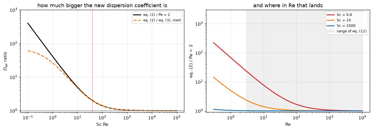
D_ax(eq. 2) = 2 D_ax(Pe = 2) at Sc Re = 40: Re = 66.7 for a gas at Sc = 0.6, Re = 0.04 for a liquid at Sc = 1000
against the INERT coefficient of eq. (3) the stagnant terms differ by a factor 71.4 (20 against 0.28 at eps_b = 0.4)
2. What that does to the reported Sherwood number
Take a bed that obeys eq. (12), run it forward through eq. (7) with the eq. (2) dispersion coefficient to get the outlet such a bed would produce, then invert eq. (8) on that outlet, which is what the original investigators did. The ratio \(\mathrm{Sh}/\mathrm{Sh}'\) is the error the paper corrects; its only free parameter is the bed height.
fig, axes = plt.subplots(1, 2, figsize=(11.8, 4.3))
Re_g = np.logspace(np.log10(3), 4, 70)
ax = axes[0]
for L_dp, ls in ((2.0, ":"), (5.0, "--"), (10.0, "-")):
    for sc, col, ph in ((C0["sc_fig2"], "tab:red", "gas"), (SC_LIQ, "tab:blue", "liquid")):
        ax.semilogx(Re_g, [correction_factor(x, sc, L_dp, C0) for x in Re_g], ls, color=col,
                    lw=1.8, label=f"{ph}, $L/d_p$ = {L_dp:g}")
ax.axhline(1.0, color="k", lw=1.2)
ax.set(xlabel="Re", ylabel=r"$\mathrm{Sh}/\mathrm{Sh}'$", ylim=(0.9, 4),
       title=f"the size of the correction (Sc = {C0['sc_fig2']} red, {SC_LIQ:g} blue)")
ax.legend(fontsize=7.5, ncol=2)
ax = axes[1]
Re = np.logspace(0, 4, 300)
ax.loglog(Re, eq12(Re, C0["sc_fig2"], C0), "k-", lw=2.2, label="eq. (12)")
ax.loglog(Re, eq9_ranz(Re, C0["sc_fig2"], C0), "--", color="tab:green", lw=1.8,
          label="eq. (9) Ranz-Marshall, single spheres")
ax.loglog(Re, eq11_petrovic(Re, C0["sc_fig2"], C0), "-.", color="tab:blue", lw=1.8,
          label="eq. (11) Petrovic-Thodos")
ax.axhline(2.0, color="tab:red", lw=1.4, ls=":", label="Sh = 2, the stagnant sphere")
ax.set(xlabel="Re", ylabel="Sh", ylim=(0.5, 300), title=f"each correlation as Re falls, Sc = {C0['sc_fig2']}")
ax.legend(fontsize=8, loc="upper left")
fig.tight_layout(); plt.show()

print("Sh/Sh' for a bed obeying eq. (12), L/d_p = 5:")
print(f"   {'Re':>8}{'gas':>10}{'liquid':>12}")
for x in (3, 10, 30, 100, 300, 1000, 3000):
    print(f"   {x:8}{correction_factor(x, C0['sc_fig2'], 5.0, C0):10.2f}"
          f"{correction_factor(x, SC_LIQ, 5.0, C0):12.4f}")
print(f"\nliquid (Sc = {SC_LIQ:g}): largest |Sh/Sh' - 1| over {C0['re_lo']:g} <= Re <= "
      f"{C0['re_hi']:g} ({N_RE_LIQ} log-spaced Re), by bed length:")
for L, (m, at) in A0["_cmax"].items():
    print(f"   L/d_p = {L:5g}: {100 * m:.3f} % at Re = {at:g}")
print(f"the largest correction sits at the low end of the range: "
      f"{100 * A0['liquid_correction_max']:.2f} % at L/d_p = 10, and at most "
      f"{100 * A0['liquid_correction_max_all_Ldp']:.2f} % for L/d_p up to {max(L_SWEEP):g}.")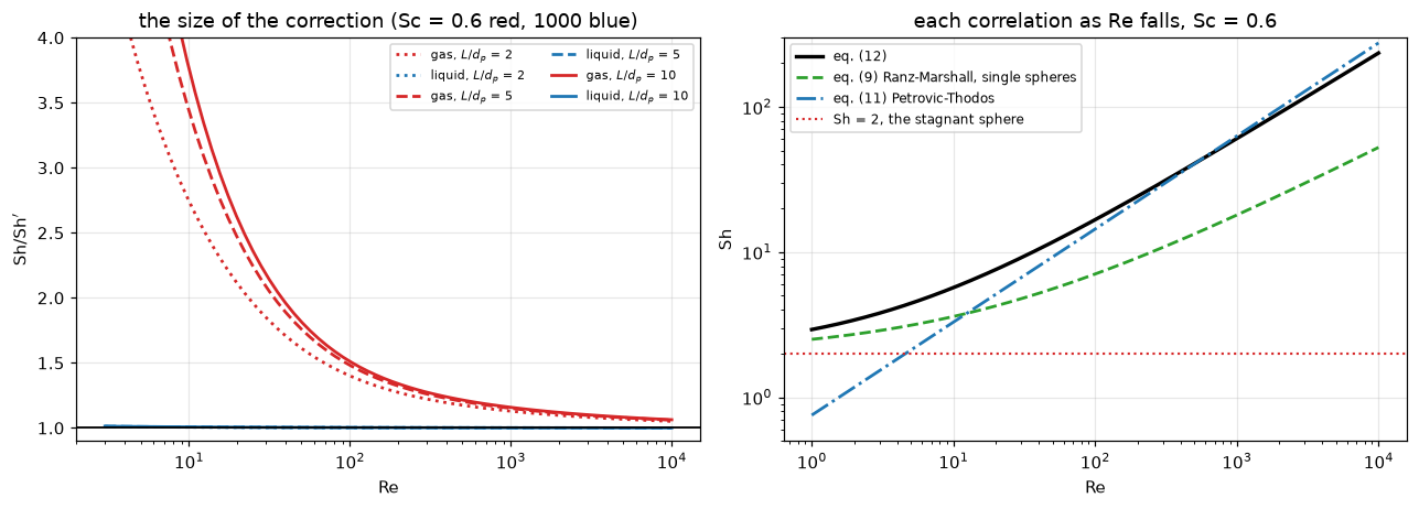
Sh/Sh' for a bed obeying eq. (12), L/d_p = 5:
         Re       gas      liquid
          3      6.92      1.0126
         10      3.44      1.0074
         30      2.09      1.0047
        100      1.48      1.0028
        300      1.26      1.0018
       1000      1.15      1.0011
       3000      1.10      1.0007

liquid (Sc = 1000): largest |Sh/Sh' - 1| over 3 <= Re <= 10000 (200 log-spaced Re), by bed length:
   L/d_p =     2: 1.054 % at Re = 3
   L/d_p =     5: 1.256 % at Re = 3
   L/d_p =    10: 1.325 % at Re = 3
   L/d_p =    20: 1.360 % at Re = 3
   L/d_p =    40: 1.378 % at Re = 3
   L/d_p =   100: 1.388 % at Re = 3
the largest correction sits at the low end of the range: 1.33 % at L/d_p = 10, and at most 1.39 % for L/d_p up to 100.
3. Redoing the paper’s own recalculation
Petrovic and Thodos’ eq. (11) is their data, already fitted, under \(\mathrm{Pe}=2\). Run it forward through eq. (7) at \(\mathrm{Pe}=2\) to recover the outlet, then invert eq. (7) again with eq. (2)’s dispersion coefficient. If Wakao and Funazkri’s arithmetic is right, what comes out should be eq. (12). Nothing is fitted: both correlations, both dispersion laws and the bed model are printed in the paper. The statistics are over a log-spaced grid of \(100 \le \mathrm{Re} \le 900\), where both correlations are inside their stated ranges.
Re_t = np.array([30, 50, 100, 200, 300, 500, 900])
print("eq. (11) re-analysed with eq. (2), against eq. (12)")
print(f"   {'Re':>6}{'eq. 11':>9}{'eq. 12':>9}" + "".join(f"{'L/dp=' + str(L):>11}" for L in (10, 20, 40)))
for x in Re_t:
    row = [(1 + reanalysis(x, C0["sc_fig2"], float(L), C0)) * eq12(x, C0["sc_fig2"], C0) for L in (10, 20, 40)]
    print(f"   {x:6}{eq11_petrovic(x, C0['sc_fig2'], C0):9.2f}{eq12(x, C0['sc_fig2'], C0):9.2f}"
          + "".join(f"{v:11.2f}" for v in row))
print(f"\nover 100 <= Re <= 900 at L/d_p = 10: mean |dev| "
      f"{100 * A0['eq11_reanalysed_vs_eq12_mean_abs_dev_logRe']:.2f} %, worst "
      f"{100 * A0['eq11_reanalysed_vs_eq12_worst']:.2f} % at Re = {A0['_worst_at_Re']:.0f}, the top of eq. (11)'s range")
print(f"L/d_p = 10 -> 40 moves the mean |dev| by {100 * A0['eq11_reanalysis_Ldp_effect_mean']:.2f} "
      f"and the worst by {100 * A0['eq11_reanalysis_Ldp_effect_worst']:.2f} percentage points; "
      f"the deviation at a single Re by at most {100 * A0['eq11_reanalysis_Ldp_effect']:.2f}")
print(f"the same re-analysis with the forward solve and the inversion both on the pymrm "
      f"discretisation ({N_PROD} cells) instead of eq. (7): largest difference "
      f"{100 * A0['reanalysis_route_gap']:.3f} percentage points at the five tabulated Re >= 100")
eq. (11) re-analysed with eq. (2), against eq. (12)
Re eq. 11 eq. 12 L/dp=10 L/dp=20 L/dp=40
30 6.66 9.14 10.68 10.98 11.14
50 9.24 11.70 12.34 12.53 12.64
100 14.41 16.70 16.54 16.65 16.71
200 22.47 24.29 23.90 23.97 24.01
300 29.14 30.43 30.27 30.32 30.35
500 40.43 40.62 41.26 41.29 41.31
900 58.93 56.95 59.50 59.53 59.54
over 100 <= Re <= 900 at L/d_p = 10: mean |dev| 1.67 %, worst 4.48 % at Re = 900, the top of eq. (11)'s range
L/d_p = 10 -> 40 moves the mean |dev| by 0.24 and the worst by 0.07 percentage points; the deviation at a single Re by at most 1.05
the same re-analysis with the forward solve and the inversion both on the pymrm discretisation (1600 cells) instead of eq. (7): largest difference 0.036 percentage points at the five tabulated Re >= 100The second route shares the correlations, the dispersion laws and the root finder with the first; it differs only in solving eq. (4) on the grid rather than using eq. (7), so its gap is the first-order discretisation error of the grid, of the size validation check 1 measures.
4. The digitised gas-phase data
Figure 2 is the paper’s own before-and-after picture: re-evaluated \(\mathrm{Sh}\) for water evaporation, with eq. (12) drawn through it, Ranz-Marshall below it and the Petrovic-Thodos line across it. Deviation is \((\text{model}-\text{measured})/\text{measured}\) throughout; a mean deviation is printed with its standard error, \(s/\sqrt{n}\).
re2, sh2, d2 = G0["_re"], G0["_sh"], G0["_d"]
Re_c = np.logspace(0, 3, 300)
fig, axes = plt.subplots(1, 2, figsize=(11.8, 4.4))
ax = axes[0]
ax.loglog(re2, sh2, "o", ms=5, mfc="none", mew=1.2, color="tab:grey",
          label=f"Figure 2, digitised ({len(re2)})")
ax.loglog(Re_c, eq12(Re_c, C0["sc_fig2"], C0), "k-", lw=2.2, label="eq. (12)")
ax.loglog(Re_c, eq9_ranz(Re_c, C0["sc_fig2"], C0), "--", color="tab:green", lw=1.7, label="eq. (9)")
ax.loglog(Re_c, eq11_petrovic(Re_c, C0["sc_fig2"], C0), "-.", color="tab:blue", lw=1.7, label="eq. (11)")
ax.set(xlabel="Re", ylabel="Sh", title="Figure 2 rebuilt from the extracted points", ylim=(1, 300))
ax.legend(fontsize=8, loc="upper left")
ax = axes[1]
for k, c, m in (("eq12", "k", "o"), ("eq11", "tab:blue", "s"), ("eq9", "tab:green", "^")):
    ax.semilogx(re2, d2[k], m, ms=4.5, mfc="none", mew=1.1, color=c, label=k.replace("eq", "eq. ("))
ax.axhline(0, color="k", lw=1.2)
ax.set(xlabel="Re", ylabel="(model - measured) / measured", ylim=(-0.9, 1.2),
       title="deviation, one convention throughout")
ax.legend(fontsize=8)
fig.tight_layout(); plt.show()

print(f"against the {G0['n_fig2_markers']} digitised markers:")
for k, lab in (("eq12", "eq. (12) this paper"), ("eq11", "eq. (11) Petrovic-T"), ("eq9", "eq.  (9) Ranz-Marsh")):
    print(f"   {lab}: mean |dev| {100 * np.abs(d2[k]).mean():5.1f} %   bias "
          f"{100 * G0[k + '_vs_fig2_bias']:+6.1f} +/- {100 * G0[k + '_vs_fig2_bias_se']:.1f} %")
print("\nbias by Reynolds band:")
print(f"   {'Re band':>14}{'n':>4}{'eq. 12':>10}{'eq. 11':>10}{'eq. 9':>10}")
for i, (lo, hi) in enumerate(GAS_BANDS):
    n = G0["_bands"]["eq12"][i][0]
    print(f"   {str(lo) + '-' + str(hi):>14}{n:4d}" +
          "".join(f"{100 * G0['_bands'][k][i][1]:+9.1f}%" for k in ("eq12", "eq11", "eq9")))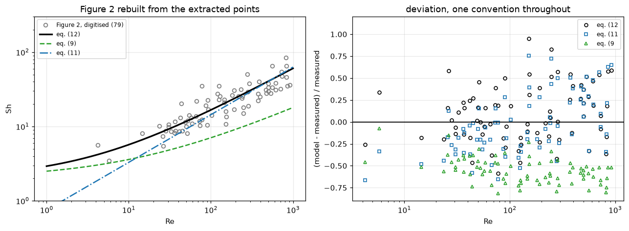
against the 79 digitised markers:
   eq. (12) this paper: mean |dev|  27.2 %   bias   +9.7 +/- 3.6 %
   eq. (11) Petrovic-T: mean |dev|  28.7 %   bias   -3.1 +/- 3.9 %
   eq.  (9) Ranz-Marsh: mean |dev|  55.1 %   bias  -55.1 +/- 1.6 %

bias by Reynolds band:
          Re band   n    eq. 12    eq. 11     eq. 9
             1-30   7     +6.7%    -31.9%    -37.2%
           30-100  27     +1.4%    -19.3%    -52.2%
          100-300  23     +8.5%     -0.3%    -58.7%
         300-1100  22    +22.2%    +22.8%    -60.7%
5. The correlation against the data it was fitted to
Figure 2 is a check; Figure 3 is the fit. Its ordinate is already \((\mathrm{Sh}-2)/\mathrm{Sc}^{1/3}\), so fitting \(y = \alpha\,\mathrm{Re}^{\beta}\) to the digitised markers is a direct test of the two printed constants. A refit of a digitised figure has three uncertainties beyond the standard error a regression prints:
- the axes may be mis-calibrated, and this figure carries its own control, the correlation drawn inside it;
- the marker set depends on how much of that drawn line is erased before detection;
- the estimator: a straight line in log-log (equal weight to every relative deviation) and a least-squares fit in linear \(y\) (dominated by the large values, the high-\(\mathrm{Re}\) end) answer different questions.
5a. The calibration, checked against a curve whose answer is known. Trace the drawn line’s ink, invert the axis calibration, fit a power law to it: the answer must be \(1.1\) and \(0.6\), and anything else is calibration error measured on an object with no scientific content. The two vertical axes of the render disagree (the decade ticks on the left sit higher than those on the right), so a single averaged origin is right in the middle of the plot and wrong at both ends; the shipped calibration interpolates the origin and the decade height in the column.
re_line, off_f, off_s = L0["_line_off"]
print(f"tick skew: y = 1 sits {L0['fig3_tick_skew_px']:+.2f} px lower under the right axis than "
      f"under the left, a rotation of {L0['fig3_rotation_deg']:.3f} degrees")
print(f"\ndrawn ink minus computed position of {C0['alpha']} Re^{C0['beta']}, {len(line3)} traced columns")
print(f"   {'Re band':>14}{'n':>5}{'flat cal.':>12}{'skew cal.':>12}")
for lo, hi in ((3, 10), (10, 100), (100, 1000), (1000, 10000)):
    m = (re_line >= lo) & (re_line < hi)
    if m.sum() >= 5:
        print(f"   {str(lo) + '-' + str(hi):>14}{m.sum():5d}{off_f[m].mean():+10.2f} px{off_s[m].mean():+10.2f} px")
print(f"   spread about the mean: {L0['fig3_line_offset_sd_flat_px']:.2f} px flat, "
      f"{L0['fig3_line_offset_sd_skew_px']:.2f} px skew-corrected")
print(f"\nthe drawn correlation refitted from its own ink ({L0['_nbin']} column bins); "
      f"the answer is alpha = {C0['alpha']}, beta = {C0['beta']}")
for lab, k in (("flat", "flat"), ("skew-corrected", "skew")):
    a, b = L0[f"fig3_drawn_line_alpha_{k}"], L0[f"fig3_drawn_line_beta_{k}"]
    print(f"   {lab:>16}: alpha {a:.4f} ({100 * (a / C0['alpha'] - 1):+.1f} %), "
          f"beta {b:.4f} ({100 * (b / C0['beta'] - 1):+.1f} %)")
tick skew: y = 1 sits +5.64 px lower under the right axis than under the left, a rotation of 0.203 degrees
drawn ink minus computed position of 1.1 Re^0.6, 410 traced columns
Re band n flat cal. skew cal.
3-10 98 -3.37 px -1.53 px
10-100 34 +0.67 px +0.97 px
100-1000 131 +2.34 px +1.98 px
1000-10000 128 +0.12 px -1.10 px
spread about the mean: 3.83 px flat, 3.54 px skew-corrected
the drawn correlation refitted from its own ink (10 column bins); the answer is alpha = 1.1, beta = 0.6
flat: alpha 1.1262 (+2.4 %), beta 0.5949 (-0.9 %)
skew-corrected: alpha 1.1073 (+0.7 %), beta 0.5984 (-0.3 %)With the skew corrected the control comes back close to the printed pair; what is left is of the order of the drawn stroke’s own scatter about a power law, which the sidecar measures. The correction moves the marker fit in the same direction (the next cells).
5b. The erasure band. Figure 3’s markers merge into chains along the drawn correlation, and the detector cannot see them until that line is erased. Most of it goes by morphology, but the remainder is removed by computed position, in a band of chosen half-width around \(1.1\,\mathrm{Re}^{0.6}\). That band is the one step that can destroy a real marker, and its width is a free choice, so the answer is reported as a function of it. “on line” counts fitted centres within 5 px of the computed line.
print(f"   {'band':>6}{'n':>5}{'alpha':>9}{'beta':>9}{'a (lin.)':>10}{'b (lin.)':>10}"
      f"{'a | b fixed':>12}{'(flat)':>9}{'on line':>9}")
for hw, v in L0["_sweep"].items():
    star = " <- shipped" if hw == BAND_SHIPPED else ""
    print(f"   {hw:6d}{v['n']:5d}{v['a']:9.4f}{v['b']:9.4f}{v['la']:10.4f}{v['lb']:10.4f}"
          f"{v['af']:12.4f}{v['aff']:9.4f}{v['on']:9d}{star}")
print(f"\nswitching the band off gains {L0['band_off_gained']} centres more than {MATCH} px from every "
      f"shipped one; their median distance from the drawn line is "
      f"{L0['band_off_gained_median_line_px']:.1f} px and their median fit score "
      f"{L0['band_off_gained_median_score']:.3f}, against {L0['shipped_median_score']:.3f} for the shipped set")
print(f"\nacross the sweep: free alpha {L0['refit_liquid_alpha_band_lo']:.3f} to "
      f"{L0['refit_liquid_alpha_band_hi']:.3f}, free beta {L0['refit_liquid_beta_band_lo']:.4f} to "
      f"{L0['refit_liquid_beta_band_hi']:.4f}")
print(f"alpha at beta = {C0['beta']}, six bands x two calibrations, log metric: "
      f"{L0['refit_liquid_alpha_beta_fixed_logmetric_lo']:.4f} to {L0['refit_liquid_alpha_beta_fixed_logmetric_hi']:.4f}")
print(f"   and over three estimators as well: {L0['refit_liquid_alpha_beta_fixed_grid_lo']:.4f} to "
      f"{L0['refit_liquid_alpha_beta_fixed_grid_hi']:.4f} "
      f"({100 * (L0['refit_liquid_alpha_beta_fixed_grid_lo'] / C0['alpha'] - 1):+.1f} % to "
      f"{100 * (L0['refit_liquid_alpha_beta_fixed_grid_hi'] / C0['alpha'] - 1):+.1f} % of {C0['alpha']})")
print(f"free alpha over the same grid: {L0['refit_liquid_alpha_free_grid_lo']:.4f} to "
      f"{L0['refit_liquid_alpha_free_grid_hi']:.4f} "
      f"({100 * (L0['refit_liquid_alpha_free_grid_lo'] / C0['alpha'] - 1):+.1f} % to "
      f"{100 * (L0['refit_liquid_alpha_free_grid_hi'] / C0['alpha'] - 1):+.1f} %)")
band n alpha beta a (lin.) b (lin.) a | b fixed (flat) on line
0 210 1.2959 0.5588 1.0513 0.6013 1.0981 1.1008 28
3 195 1.3275 0.5526 1.1616 0.5837 1.0977 1.1004 17
5 182 1.3437 0.5496 1.1567 0.5844 1.1000 1.1029 3 <- shipped
7 166 1.3596 0.5466 1.1651 0.5822 1.1010 1.1040 0
10 147 1.4169 0.5361 1.2146 0.5727 1.1061 1.1094 0
14 126 1.4401 0.5328 1.2287 0.5718 1.1143 1.1179 0
switching the band off gains 32 centres more than 6.7 px from every shipped one; their median distance from the drawn line is 2.9 px and their median fit score 0.692, against 0.793 for the shipped set
across the sweep: free alpha 1.296 to 1.440, free beta 0.5328 to 0.5588
alpha at beta = 0.6, six bands x two calibrations, log metric: 1.0977 to 1.1179
and over three estimators as well: 1.0067 to 1.1179 (-8.5 % to +1.6 % of 1.1)
free alpha over the same grid: 1.0513 to 1.4648 (-4.4 % to +33.2 %)Erasing more of the line removes the markers lying on it, the ones nearest the printed correlation, so \(\alpha\) climbs and \(\beta\) falls as the band widens. The shipped setting is mid-range: switching the band off finds more centres, but they sit on the drawn line and score worse than the shipped set (both medians above), so they are more likely surviving fragments of the line than rescued markers. That is a judgement; its cost if wrong is the width of the sweep.
One number barely moves: \(\alpha\) with \(\beta\) held at the printed value, across the whole sweep and both calibrations, while the free \(\alpha\) moves by tens of per cent. It is not a fixed point: the estimator and the starting \(\mathrm{Re}\) both move it by a few per cent, and the next cell prints both.
fam = L0["_fam"]
print(f"the fit family on the shipped set: {L0['n_fig3_markers']} markers; printed alpha = "
      f"{C0['alpha']}, beta = {C0['beta']}")
print(f"   {'calibration':>12}{'estimator':>28}{'alpha':>10}{'beta':>10}")
for cal_name in ("flat", "skew"):
    for k, lab in (("log", "least squares in log y"), ("lin", "least squares in linear y"),
                   ("ts", "Theil-Sen in log y")):
        print(f"   {cal_name:>12}{lab:>28}{fam[(cal_name, k)][0]:10.4f}{fam[(cal_name, k)][1]:10.4f}")
    for h, lab in (("log", "beta fixed: geometric mean"), ("lin", "beta fixed: linear-y LS"),
                   ("med", "beta fixed: median ratio")):
        print(f"   {cal_name:>12}{lab:>28}{fam[(cal_name, 'fix', h)]:10.4f}{C0['beta']:10.4f}")
print("\nthe log-space fit, started at increasing Reynolds number (skew calibration):")
print(f"   {'Re >=':>7}{'n':>5}{'alpha':>9}{'beta':>9}{'a | b fixed':>13}")
for c0, (n, a, b, af) in L0["_cut"].items():
    print(f"   {c0:7d}{n:5d}{a:9.3f}{b:9.4f}{af:13.4f}")
the fit family on the shipped set: 182 markers; printed alpha = 1.1, beta = 0.6
calibration estimator alpha beta
flat least squares in log y 1.3667 0.5460
flat least squares in linear y 1.1723 0.5815
flat Theil-Sen in log y 1.2118 0.5521
flat beta fixed: geometric mean 1.1029 0.6000
flat beta fixed: linear-y LS 1.0411 0.6000
flat beta fixed: median ratio 1.0529 0.6000
skew least squares in log y 1.3437 0.5496
skew least squares in linear y 1.1567 0.5844
skew Theil-Sen in log y 1.1899 0.5558
skew beta fixed: geometric mean 1.1000 0.6000
skew beta fixed: linear-y LS 1.0469 0.6000
skew beta fixed: median ratio 1.0518 0.6000
the log-space fit, started at increasing Reynolds number (skew calibration):
Re >= n alpha beta a | b fixed
3 182 1.344 0.5496 1.1000
5 164 1.181 0.5753 1.0629
10 145 1.112 0.5866 1.0464
20 125 1.009 0.6045 1.0315
30 114 0.995 0.6070 1.0304
50 91 0.861 0.6316 1.01995c. The estimator. Within each block of that table the rows are the same markers and the same model under different loss functions, and they disagree by more than either differs from the printed pair. The paper does not say which it used. Its Figure 4, where it pools gas and liquid data against \((\mathrm{Sc}^{1/3}\mathrm{Re}^{0.6})^2\) and writes “it is seen that the data are well correlated by eqn (12)”, is drawn on log-log axes like every figure in the paper, and the square is taken “to enlarge the plot in the x-axis direction”: a presentational choice, not a weighting. A two-significant-figure correlation drawn through data pooled from thirty-eight sources does not have a recoverable loss function.
5d. The standard errors. The ordinary least-squares errors assume independent, identically distributed residuals. The markers come from eleven laboratories, each covering a window in \(\mathrm{Re}\) with its own offset, and a straight line in log-log may not be the right mean function. Both are measurable: a quadratic term with its \(t\) value, the residual autocorrelation in \(\mathrm{Re}\) order (its standard error is about \(1/\sqrt{n}\)), Newey-West errors, and a bootstrap that resamples whole \(\mathrm{Re}\) bins.
q, qse, qdof = L0["_quad"]
n_l = L0["n_fig3_markers"]
print(f"quadratic term in log-log: {q:+.4f} +/- {qse:.4f}, t = {L0['refit_liquid_quadratic_term_z']:.1f} "
      f"on {qdof} degrees of freedom ({n_l} markers, three coefficients)")
print("residual autocorrelation in log-Re order: " +
      ", ".join(f"lag {L} {v:+.2f}" for L, v in L0["_acf"].items()) +
      f"   (1/sqrt(n) = {1 / np.sqrt(n_l):.2f})")
a, b = L0["refit_liquid_alpha"], L0["refit_liquid_beta"]
print(f"\nthe free log-log fit, alpha = {a:.3f} / beta = {b:.4f}, {n_l} markers, {L0['_dof1']} degrees "
      f"of freedom; z is the distance from the printed value in standard errors")
print(f"   {'error model':>34}{'SE(alpha)':>11}{'SE(beta)':>11}{'z(alpha)':>10}{'z(beta)':>9}")
rows_err = [("ordinary least squares (iid)", L0["refit_liquid_alpha_se"], L0["refit_liquid_beta_se"])]
rows_err += [(f"Newey-West, {L} lags", *v) for L, v in L0["_hac"].items()]
rows_err += [(f"bootstrap of {L0['_n_clusters']} Re bins", L0["refit_liquid_alpha_se_cluster"],
              L0["refit_liquid_beta_se_cluster"])]
for lab, sa, sb in rows_err:
    print(f"   {lab:>34}{sa:11.4f}{sb:11.4f}{abs(a - C0['alpha']) / sa:10.1f}{abs(b - C0['beta']) / sb:9.1f}")
print(f"\n   bin bootstrap ({DRAWS} draws) 95 % interval: alpha {L0['refit_liquid_alpha_cluster_ci_lo']:.3f} "
      f"to {L0['refit_liquid_alpha_cluster_ci_hi']:.3f}, beta {L0['refit_liquid_beta_cluster_ci_lo']:.4f} "
      f"to {L0['refit_liquid_beta_cluster_ci_hi']:.4f}")
print(f"   the erasure band alone spans a half-width of "
      f"{0.5 * (L0['refit_liquid_alpha_band_hi'] - L0['refit_liquid_alpha_band_lo']):.3f} in alpha: "
      f"{L0['band_halfwidth_over_iid_se']:.1f} iid standard errors, "
      f"{L0['band_halfwidth_over_cluster_se']:.2f} bin-bootstrap ones")
quadratic term in log-log: +0.0558 +/- 0.0111, t = 5.0 on 179 degrees of freedom (182 markers, three coefficients)
residual autocorrelation in log-Re order: lag 1 +0.04, lag 2 +0.09, lag 3 +0.11, lag 5 +0.12, lag 10 +0.12 (1/sqrt(n) = 0.07)
the free log-log fit, alpha = 1.344 / beta = 0.5496, 182 markers, 180 degrees of freedom; z is the distance from the printed value in standard errors
error model SE(alpha) SE(beta) z(alpha) z(beta)
ordinary least squares (iid) 0.0520 0.0090 4.7 5.6
Newey-West, 5 lags 0.0740 0.0121 3.3 4.2
Newey-West, 10 lags 0.0882 0.0145 2.8 3.5
Newey-West, 20 lags 0.0995 0.0169 2.5 3.0
bootstrap of 9 Re bins 0.1319 0.0229 1.8 2.2
bin bootstrap (20000 draws) 95 % interval: alpha 1.041 to 1.531, beta 0.5082 to 0.5988
the erasure band alone spans a half-width of 0.072 in alpha: 1.4 iid standard errors, 0.55 bin-bootstrap onesSo what survives?
The printed pair is not rejected by this figure. The bin-bootstrap interval on \(\alpha\) contains the printed value; the one on \(\beta\) ends at it, to a tenth of a bootstrap standard error, and the linear-metric fit returns a \(\beta\) inside it. The extraction band alone moves \(\alpha\) by more than the iid standard error and by about half the bootstrap one.
What survives is that the figure returns the printed \(\alpha\) once \(\beta\) is held at its printed value, within a few per cent under every band, calibration and estimator tried, while the free \(\alpha\) runs up to a third high. Two things move the \(\beta\)-fixed \(\alpha\), and both are printed: the estimator, and the starting \(\mathrm{Re}\).
And a weaker statement about shape. The free exponent is below the printed one under every estimator on the shipped set, because the markers at the lowest \(\mathrm{Re}\) sit above the drawn line; as they are dropped the fit walks through the printed pair (the starting-\(\mathrm{Re}\) table). The paper sets aside liquid data below \(\mathrm{Re}\approx 3\) as possibly affected by natural convection, which inflates the coefficient; the binned deviations below show the excess has not finished by \(\mathrm{Re}=3\). The quadratic term says a two-parameter power law is not the right description of this cloud in the first place.
dev3, re_s, y_s = L0["_dev"], L0["_re_s"], L0["_y_s"]
fig, axes = plt.subplots(1, 2, figsize=(11.8, 4.4))
Re_l = np.logspace(np.log10(2.5), np.log10(3500), 300)
ax = axes[0]
ax.loglog(re_s, y_s, "o", ms=4, mfc="none", mew=1.0, color="tab:blue", label=f"Figure 3, digitised ({len(re_s)})")
ax.loglog(Re_l, C0["alpha"] * Re_l ** C0["beta"], "k-", lw=2.2, label="printed")
ax.loglog(Re_l, L0["refit_liquid_alpha_beta_fixed"] * Re_l ** C0["beta"], "-", color="tab:orange", lw=1.6,
          label="beta held, alpha fitted")
ax.loglog(Re_l, a * Re_l ** b, "--", color="tab:red", lw=1.8, label="free, log metric")
ax.loglog(Re_l, L0["refit_liquid_alpha_linear_metric"] * Re_l ** L0["refit_liquid_beta_linear_metric"],
          ":", color="tab:green", lw=2.0, label="free, linear metric")
ax.set(xlabel="Re", ylabel=r"$(\mathrm{Sh}-2)/\mathrm{Sc}^{1/3}$",
       title="Figure 3 rebuilt: the data alpha and beta were fitted on")
ax.legend(fontsize=7.5, loc="upper left")
ax = axes[1]
ax.semilogx(re_s, dev3, "o", ms=4, mfc="none", mew=1.0, color="tab:blue")
ax.axhline(0, color="k", lw=1.2)
bn = L0["_binned"]
ax.errorbar([np.sqrt(lo * hi) for lo, hi, *_ in bn], [m for *_, m, s in bn], [s for *_, s in bn],
            fmt="s-", color="tab:red", lw=2, ms=6, label="binned mean +/- standard error")
ax.set(xlabel="Re", ylabel="(model - measured) / measured", ylim=(-0.6, 0.6),
       title="deviation of the PRINTED correlation from its own data")
ax.legend(fontsize=8)
fig.tight_layout(); plt.show()

print(f"eq. (12) against the {len(re_s)} liquid markers: mean |dev| {100 * L0['eq12_vs_fig3_mean_abs_dev']:.1f} %, "
      f"bias {100 * L0['eq12_vs_fig3_bias']:+.1f} +/- {100 * L0['eq12_vs_fig3_bias_se']:.1f} %")
print(f"eq. (12) against the {G0['n_fig2_markers']} gas markers: mean |dev| "
      f"{100 * G0['eq12_vs_fig2_mean_abs_dev']:.1f} %, bias {100 * G0['eq12_vs_fig2_bias']:+.1f} +/- "
      f"{100 * G0['eq12_vs_fig2_bias_se']:.1f} %")
print(f"\n   {'Re band':>14}{'n':>5}{'mean dev':>11}{'SE':>7}")
for lo, hi, n, m, s in bn:
    print(f"   {str(int(lo)) + '-' + str(int(hi)):>14}{n:5d}{100 * m:+10.1f}%{100 * s:6.1f}%")
print(f"the markers lie {100 * L0['fig3_excess_3_6']:.0f} % above the drawn line for 3 <= Re < 6 "
      f"({L0['fig3_excess_3_6_z']:.1f} standard errors) and {100 * L0['fig3_excess_6_12']:.0f} % for "
      f"6 <= Re < 12 ({L0['fig3_excess_6_12_z']:.1f})")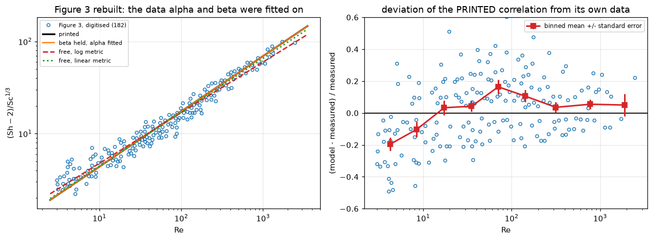
eq. (12) against the 182 liquid markers: mean |dev| 17.6 %, bias +2.3 +/- 1.6 %
eq. (12) against the 79 gas markers: mean |dev| 27.2 %, bias +9.7 +/- 3.6 %

          Re band    n   mean dev     SE
              3-6   23     -19.6%   4.1%
             6-12   17     -10.3%   4.7%
            12-25   21      +3.3%   4.6%
            25-50   30      +4.2%   3.4%
           50-100   25     +16.4%   4.3%
          100-200   23     +10.7%   3.9%
          200-500   23      +3.6%   3.3%
         500-1200   16      +5.5%   3.1%
        1200-3000    4      +5.0%   7.0%
the markers lie 24 % above the drawn line for 3 <= Re < 6 (4.7 standard errors) and 11 % for 6 <= Re < 12 (2.2)
Validation
Seven checks. The first three involve no data. A break table at the end injects a defect into every input the claims depend on and records which claims catch it.
1. pymrm against eq. (7). The paper’s closed form is the exact solution of the problem pymrm discretises, so refinement must converge onto it. The cases are solved on a nested ladder of uniform grids; orders come from successive differences of three levels (pymrm.checks.observed_orders), which need no exact solution, and the Richardson value extrapolated with the observed order of the finest triple is compared with eq. (7). Upwind convection is first order. The round-off companion is the finest successive difference divided by the relative residual of the linear solve: the orders are read far above round-off.
print(f"ladder {LADDER} cells")
for r in B0["_rows"]:
    print(f"   N = {r['N']:5.1f}, Pe_L = {r['Pe']:5.1f}: error {r['err'][0]:+.2e} -> {r['err'][-1]:+.2e}, "
          f"orders {', '.join(f'{o:.4f}' for o in r['orders'])}, extrapolated {r['extrap']:+.1e}, "
          f"solve residual below 1e-11 (here {r['resid']:.0e})")
print(f"orders {B0['pymrm_order_min']:.4f} to {B0['pymrm_order_max']:.4f} (first order); "
      f"largest error at {N_PROD} cells {B0['pymrm_vs_eq7_n1600']:.2e}; the extrapolated value is "
      f"below 1e-5 from eq. (7) (here {B0['pymrm_vs_eq7_richardson']:.1e}); the finest difference is "
      f"more than 1e3 times the solve residual (here {B0['pymrm_finest_diff_over_residual']:.0e})")
ladder (200, 400, 800, 1600, 3200) cells
N = 1.0, Pe_L = 40.0: error +2.16e-03 -> +1.35e-04, orders 0.9969, 0.9984, 0.9992, extrapolated -9.8e-08, solve residual below 1e-11 (here 3e-14)
N = 5.0, Pe_L = 10.0: error +1.72e-02 -> +1.07e-03, orders 1.0074, 1.0038, 1.0019, extrapolated +1.9e-06, solve residual below 1e-11 (here 1e-13)
N = 0.5, Pe_L = 4.0: error +2.48e-04 -> +1.55e-05, orders 0.9988, 0.9994, 0.9997, extrapolated -3.8e-09, solve residual below 1e-11 (here 3e-13)
N = 20.0, Pe_L = 2.0: error +9.87e-03 -> +6.02e-04, orders 1.0280, 1.0142, 1.0071, extrapolated +3.9e-06, solve residual below 1e-11 (here 1e-13)
orders 0.9969 to 1.0280 (first order); largest error at 1600 cells 2.14e-03; the extrapolated value is below 1e-5 from eq. (7) (here 3.9e-06); the finest difference is more than 1e3 times the solve residual (here 5e+07)2. Eq. (7) collapses onto eq. (8) when the dispersion is switched off. The paper says “eqn (7) reduces to eqn (8), when not only \(D_{ax}=0\) but also Sc Re is sufficiently large”, and that is why the liquid data survive. Expanding eq. (7) for large \(\mathrm{Pe}_L\) gives \(\ln(\theta_7/\theta_8) \approx N^2/\mathrm{Pe}_L\), so the scaled gap \(\ln(\theta_7/\theta_8)\,\mathrm{Pe}_L/N^2\) must tend to one. Result 2 already printed what it means for a liquid bed.
N = 2.0
for Pe in (2, 10, 50, 200, 1e3, 1e4, 1e5):
    r = theta_eq7(N, Pe) / theta_eq8(N)
    print(f"   Pe_L = {Pe:8.0f}: eq. 7 / eq. 8 = {r:.6f}   ln(ratio) Pe_L / N^2 = {np.log(r) * Pe / N ** 2:.5f}")
Pe_L = 2: eq. 7 / eq. 8 = 1.836562 ln(ratio) Pe_L / N^2 = 0.30395
Pe_L = 10: eq. 7 / eq. 8 = 1.310331 ln(ratio) Pe_L / N^2 = 0.67570
Pe_L = 50: eq. 7 / eq. 8 = 1.075515 ln(ratio) Pe_L / N^2 = 0.90999
Pe_L = 200: eq. 7 / eq. 8 = 1.019705 ln(ratio) Pe_L / N^2 = 0.97568
Pe_L = 1000: eq. 7 / eq. 8 = 1.003988 ln(ratio) Pe_L / N^2 = 0.99503
Pe_L = 10000: eq. 7 / eq. 8 = 1.000400 ln(ratio) Pe_L / N^2 = 0.99950
Pe_L = 100000: eq. 7 / eq. 8 = 1.000040 ln(ratio) Pe_L / N^2 = 0.999953. The stagnant-sphere limit. Eq. (12) was written as \(2 + \alpha\,\mathrm{Sc}^{1/3}\mathrm{Re}^{\beta}\) so that it cannot fall below 2, for any \(\alpha\) and positive \(\beta\): an identity of the form, which cannot fail. Eq. (11) has no such floor; where it crosses \(\mathrm{Sh} = 2\) is a root over \(10^{-6} \le \mathrm{Re} \le 10^6\).
print(f"   {'Re':>10}{'eq. 12':>10}{'eq. 9':>10}{'eq. 11':>10}")
for x in (10.0, 1.0, 0.1, 0.01, 1e-3, 1e-6):
    print(f"   {x:10.0e}{eq12(x, C0['sc_fig2'], C0):10.4f}{eq9_ranz(x, C0['sc_fig2'], C0):10.4f}"
          f"{eq11_petrovic(x, C0['sc_fig2'], C0):10.4f}")
SH_LIMIT = max(abs(eq12(1e-30, C0["sc_fig2"], C0) - 2.0), abs(eq9_ranz(1e-30, C0["sc_fig2"], C0) - 2.0))
print(f"eq. (12) and eq. (9) at Re = 1e-30 differ from 2 by below 1e-12 (here {SH_LIMIT:.1e}); "
      f"eq. (11) crosses Sh = 2 at Re = {A0['eq11_crosses_sh2_Re']:.2f} and keeps falling")
Re eq. 12 eq. 9 eq. 11
1e+01 5.6935 3.6003 3.2935
1e+00 2.9278 2.5061 0.7528
1e-01 2.2330 2.1600 0.1721
1e-02 2.0585 2.0506 0.0393
1e-03 2.0147 2.0160 0.0090
1e-06 2.0002 2.0005 0.0001
eq. (12) and eq. (9) at Re = 1e-30 differ from 2 by below 1e-12 (here 4.4e-16); eq. (11) crosses Sh = 2 at Re = 4.59 and keeps falling4. Figure 2’s calibration. All three curves on Figure 2 are known functions, so recomputing them on the source image tests the axes (the sidecar records the overlay). Two of the three are genuinely known; eq. (11) contains \(\varepsilon_b\), which was fitted to the very line it is checked against, so it constrains the calibration in slope only. The sidecar also records the ink of all three curves sitting slightly above their computed rows, all the same way; that offset is not corrected, because the only evidence for it is those three curves, one of which supplied \(\varepsilon_b\). The cell prints the sidecar’s measurement and what one pixel of ordinate origin is worth.
Eq. (9) is drawn dashed, and its dashes are compact ink a shape test cannot tell from a marker, so they were erased by computed position: the one step that can destroy a Figure 2 marker. How many surviving markers lie near that band is countable.
print(META["fig2"]["calibration_check"]["residual_offset"])
print(f"one pixel of Figure 2's ordinate origin is {100 * G0['fig2_sh_per_px']:.2f} % in every Sh")
d9 = G0["_d9"]
print(f"\nmarkers by distance from the computed eq. (9) curve (erased band +/- {DASH_HW:.0f} px):")
for w in (DASH_HW, 15.0, 20.0, 30.0, 50.0):
    print(f"   within {w:4.0f} px: {int((d9 <= w).sum()):3d} of {len(d9)}")
print(f"nearest marker {G0['fig2_eq9_nearest_px']:.1f} px away; {G0['fig2_markers_Re_1_30']} markers in "
      f"1 <= Re <= 30, where the cloud crosses that curve. With the {G0['_n_within_50']} markers inside "
      f"50 px spread evenly in distance, the band would hold {G0['fig2_eq9_expected_in_band']:.2f} on "
      f"average, so finding none is the likelier outcome even if the band destroyed nothing.")
Measured 2026-08-02 by `setup2.trace_curves`, which takes the ink centroid column by column wherever the straight ink near the computed curve is a single run no wider than 8 px (that filter is what keeps markers sitting on a curve out of the measurement). Drawn ink minus computed row, negative meaning the ink is ABOVE the computed position:
eq. (12) n = 701 -4.06 +/- 2.30 px = +2.80 % in Sh
eq. (11) n = 582 -5.06 +/- 1.89 px = +3.51 % in Sh
eq. (9) n = 206 -2.08 +/- 6.27 px = +1.43 % in Sh
Each is inside a line width on its own; all three the SAME WAY is an ordinate origin about 4 px low, which makes every extracted Sh in this file roughly 2.7 % high and moves the page's +9.7 % eq. (12) bias to about +12.7 %. NOT CORRECTED, deliberately: the only evidence for it is those three drawn curves, one of which supplied eps_b, so correcting the ordinate on it would make this whole check circular. Contrast Figure 3, where the analogous skew is measured on eight printed decade ticks and the drawn line is an independent control - there it IS corrected.
one pixel of Figure 2's ordinate origin is 0.68 % in every Sh
markers by distance from the computed eq. (9) curve (erased band +/- 9 px):
within 9 px: 0 of 79
within 15 px: 1 of 79
within 20 px: 1 of 79
within 30 px: 2 of 79
within 50 px: 3 of 79
nearest marker 11.7 px away; 7 markers in 1 <= Re <= 30, where the cloud crosses that curve. With the 3 markers inside 50 px spread evenly in distance, the band would hold 0.54 on average, so finding none is the likelier outcome even if the band destroyed nothing.5. The correlation refitted freely from both figures. On Figure 2 the form \(\mathrm{Sh} = 2 + a\,\mathrm{Sc}^{1/3}\mathrm{Re}^{b}\) is fitted with each residual divided by the measured \(\mathrm{Sh}\) (sigma = Sh), which is least squares in the relative deviation, the same weighting as the log-log fit on Figure 3. Both standard errors are iid ones, scaled by the residual variance on \(n-2\) degrees of freedom, and optimistic for the reason 5d measures; the ratio of the two is what says which figure is the sharper instrument.
print(f"Figure 2, {G0['n_fig2_markers']} gas markers, {G0['_gas_dof']} degrees of freedom: "
      f"a = {G0['refit_gas_alpha']:.3f} +/- {G0['refit_gas_alpha_se']:.3f}, "
      f"b = {G0['refit_gas_beta']:.4f} +/- {G0['refit_gas_beta_se']:.4f}; the printed pair is within "
      f"{G0['refit_gas_max_z']:.2f} standard errors")
print(f"Figure 3, {L0['n_fig3_markers']} liquid markers, {L0['_dof1']} degrees of freedom: "
      f"a = {L0['refit_liquid_alpha']:.3f} +/- {L0['refit_liquid_alpha_se']:.3f}, "
      f"b = {L0['refit_liquid_beta']:.4f} +/- {L0['refit_liquid_beta_se']:.4f}")
SE_RATIO_A = G0["refit_gas_alpha_se"] / L0["refit_liquid_alpha_se"]
SE_RATIO_B = G0["refit_gas_beta_se"] / L0["refit_liquid_beta_se"]
print(f"the liquid figure's standard errors are {SE_RATIO_A:.1f} times smaller in alpha and "
      f"{SE_RATIO_B:.1f} times in beta")
Figure 2, 79 gas markers, 77 degrees of freedom: a = 1.185 +/- 0.202, b = 0.5467 +/- 0.0326; the printed pair is within 1.64 standard errors
Figure 3, 182 liquid markers, 180 degrees of freedom: a = 1.344 +/- 0.052, b = 0.5496 +/- 0.0090
the liquid figure's standard errors are 3.9 times smaller in alpha and 3.6 times in beta6. The shape of the argument. The paper says of Figure 2 that “at higher Reynolds numbers the data are satisfactorily correlated by the Petrovic-Thodos equation. However, at lower Reynolds numbers the data are obviously higher than their correlation.” That is a claim about a trend in the residual, which a digitised figure can test even when the marker count is short. The cell reduces the banded table of result 4 to one number per correlation: the change of the binned bias from the lowest Reynolds band to the highest.
for k in ("eq12", "eq11", "eq9"):
    lo_, hi_ = G0["_bands"][k][0][1], G0["_bands"][k][-1][1]
    print(f"   {k}: {100 * lo_:+6.1f} % -> {100 * hi_:+6.1f} %, change {100 * (hi_ - lo_):+6.1f} points")
print(f"eq. (11)'s bias changes {G0['fig2_span_ratio_eq11_over_eq12']:.1f} times as much across the range as "
      f"eq. (12)'s; eq. (9) is negative in {G0['eq9_bands_negative']} of {len(GAS_BANDS)} bands")
eq12: +6.7 % -> +22.2 %, change +15.5 points
eq11: -31.9 % -> +22.8 %, change +54.7 points
eq9: -37.2 % -> -60.7 %, change -23.5 points
eq. (11)'s bias changes 3.5 times as much across the range as eq. (12)'s; eq. (9) is negative in 4 of 4 bands7. What the re-centring did. The maintainer’s audit of the first extraction was “mostly symbols are identified well, but often the marker is off centre”; the shape fit followed. Figure 2’s file keeps both the first-pass crosshair and the fitted centre for every first-pass marker, so the displacement is a paired sample. A marker whose shape fit scored below the acceptance threshold keeps its crosshair (recentred = False) and has zero displacement by construction, so the displacement statistics use only the re-centred ones; the paired refit uses all.
pa, sa, pb, sb = R0["_fits"]
print(f"{R0['n_paired']} paired rows, {R0['n_recentred']} re-centred")
print(f"   along Re (columns): {R0['recentre_col_shift_px']:+.2f} px, {R0['recentre_col_shift_z']:.1f} "
      f"standard errors from zero")
print(f"   along Sh (rows):    {R0['recentre_row_shift_px']:+.2f} px, {R0['recentre_row_shift_z']:.1f} "
      f"standard errors from zero, {100 * R0['recentre_sh_shift']:+.2f} % in Sh")
print(f"   distance moved: median {R0['recentre_median_shift_px']:.2f} px, max {R0['_max_shift_px']:.2f} px")
print(f"refit on the same {R0['n_paired']} markers: crosshairs a = {pa[0]:.3f} +/- {sa[0]:.3f}, "
      f"b = {pa[1]:.4f}; fitted centres a = {pb[0]:.3f} +/- {sb[0]:.3f}, b = {pb[1]:.4f}: "
      f"{R0['recentre_alpha_shift_in_se']:.2f} and {R0['recentre_beta_shift_in_se']:.2f} standard errors apart")
sep = R0["_sep"]
print(f"\n{R0['n_double_counts']} of the {R0['n_paired']} crosshairs are a second or third mark on a glyph "
      f"another crosshair already had; {R0['n_second_pass']} markers were added by the second pass")
print("separations of the merged crosshairs: " + "  ".join(f"{v:.1f}" for v in sep) + " px")
print(f"{R0['n_merged_pairs_below_6px']} of {len(sep)} pairs are closer than 6 px, inside the 8 px non-maximum suppression "
      "the first pass documents, so that suppression does not explain the double counts; the cause is not known.")
81 paired rows, 65 re-centred
along Re (columns): -0.01 px, 0.0 standard errors from zero
along Sh (rows): +0.78 px, 2.6 standard errors from zero, -0.52 % in Sh
distance moved: median 3.29 px, max 9.88 px
refit on the same 81 markers: crosshairs a = 1.168 +/- 0.218, b = 0.5550; fitted centres a = 1.152 +/- 0.214, b = 0.5572: 0.08 and 0.06 standard errors apart
11 of the 81 crosshairs are a second or third mark on a glyph another crosshair already had; 9 markers were added by the second pass
separations of the merged crosshairs: 1.4 1.5 2.0 2.0 2.2 3.0 3.2 5.0 8.0 8.3 9.0 9.1 px
8 of 12 pairs are closer than 6 px, inside the 8 px non-maximum suppression the first pass documents, so that suppression does not explain the double counts; the cause is not known.The row displacement is a few standard errors from zero, so it is a small bias, not noise; in \(\mathrm{Sh}\) it is well under the scatter of the data, and the fitted constants move by a small fraction of a standard error. The shape fit’s other effect is that two crosshairs on one glyph produce two fits at the same point, which exposes double counting.
The conditioning limit
\(\theta_{out}\) is what the experiment measures. Where it falls below the resolution of an outlet analysis the measurement no longer constrains \(\mathrm{Sh}\), whatever dispersion coefficient is assumed. The cell takes \(10^{-3}\) as that resolution (an assumption, not a measured number) and finds where a gas bed obeying eq. (12) reaches it, as a root over the whole range of eq. (12), for two bed lengths.
print(f"   {'L/d_p':>7}{'Re':>8}{'theta_out':>13}{'d ln theta / d ln Sh':>23}")
for L_dp in (5.0, 10.0):
    for x in (3.0, 10.0, 30.0, 100.0):
        sh = eq12(x, C0["sc_fig2"], C0)
        th = theta_of_Sh(sh, x, C0["sc_fig2"], L_dp, "eq2", C0)
        th2 = theta_of_Sh(1.01 * sh, x, C0["sc_fig2"], L_dp, "eq2", C0)
        print(f"   {L_dp:7.0f}{x:8.0f}{th:13.2e}{(np.log(th2) - np.log(th)) / np.log(1.01):23.2f}")
print(f"theta_out = {SAT:g}: at L/d_p = 10 for Re below {A0['gas_saturation_Re_Ldp10']:.1f}; at L/d_p = 5 "
      f"{'nowhere' if not A0['gas_saturates_in_range_Ldp5'] else 'somewhere'} in "
      f"{C0['re_lo']:g} <= Re <= {C0['re_hi']:g} (the outlet stays at least "
      f"{np.exp(A0['_sat_min_L5']):.1f} times {SAT:g})")
L/d_p Re theta_out d ln theta / d ln Sh
5 3 4.16e-03 -2.47
5 10 6.93e-03 -2.72
5 30 1.26e-02 -2.82
5 100 3.40e-02 -2.55
10 3 9.00e-05 -4.49
10 10 1.13e-04 -5.06
10 30 2.31e-04 -5.39
10 100 1.32e-03 -4.96
theta_out = 0.001: at L/d_p = 10 for Re below 85.0; at L/d_p = 5 nowhere in 3 <= Re <= 10000 (the outlet stays at least 4.2 times 0.001)Claims
Every number the page states, with how it is checked. Closed-form algebra and least-squares fits solved exactly are held to FIXED; results of an iterative fit (curve_fit, Theil-Sen) to ITER; the bin bootstrap to three times the spread of its value over twelve seeds, measured here. Residuals, identities, orders and two-route gaps are bounds with their basis. A count decided against a threshold carries its margin, in pixels where the threshold is one.
FIXED, ITER = 1e-6, 1e-4
BOOT = ["refit_liquid_alpha_cluster_ci_lo", "refit_liquid_alpha_cluster_ci_hi",
        "refit_liquid_beta_cluster_ci_lo", "refit_liquid_beta_cluster_ci_hi",
        "refit_liquid_alpha_se_cluster", "refit_liquid_beta_se_cluster",
        "refit_liquid_cluster_se_inflation_alpha", "refit_liquid_z_alpha_cluster",
        "refit_liquid_z_beta_cluster", "band_halfwidth_over_cluster_se"]
SEEDS = [liquid_study(C0, CAL3, seed=s) for s in range(12)]
BOOT_RTOL = {k: 3 * np.std([r[k] for r in SEEDS], ddof=1) / abs(np.mean([r[k] for r in SEEDS]))
             for k in BOOT}
print("bootstrap seed spread (relative, x3): " +
      ", ".join(f"{k.replace('refit_liquid_', '')} {v:.1e}" for k, v in BOOT_RTOL.items()))

ITERATIVE = {"refit_liquid_alpha_linear_metric", "refit_liquid_beta_linear_metric",
             "refit_liquid_alpha_theil_sen", "refit_liquid_beta_theil_sen",
             "refit_liquid_alpha_free_grid_lo", "refit_liquid_alpha_free_grid_hi",
             "liquid_free_beta_max_shipped", "refit_gas_alpha", "refit_gas_beta",
             "refit_gas_alpha_se", "refit_gas_beta_se", "refit_gas_max_z",
             "recentre_alpha_shift_in_se", "recentre_beta_shift_in_se"}
VALUES = {
    "A": ["dax_double_ScRe", "dax_double_Re_gas", "dax_double_Re_liquid", "inert_stagnant_ratio",
          "liquid_correction_max", "liquid_correction_max_all_Ldp", "gas_correction_Re3_Ldp5",
          "eq11_reanalysed_vs_eq12_mean_abs_dev_logRe", "eq11_reanalysed_vs_eq12_worst",
          "eq11_reanalysis_Ldp_effect", "eq11_reanalysis_Ldp_effect_mean",
          "eq11_reanalysis_Ldp_effect_worst", "eq11_crosses_sh2_Re",
          "gas_saturation_Re_Ldp10"],
    "B": ["pymrm_vs_eq7_n1600"],
    "E": ["eq7_eq8_rate"],
    "G": ["eq12_vs_fig2_mean_abs_dev", "eq12_vs_fig2_bias", "eq12_vs_fig2_bias_se",
          "eq11_vs_fig2_bias", "eq11_vs_fig2_bias_se", "eq9_vs_fig2_bias", "eq9_vs_fig2_bias_se",
          "fig2_span_eq12", "fig2_span_eq11", "fig2_span_ratio_eq11_over_eq12", "fig2_sh_per_px",
          "fig2_eq9_nearest_px", "fig2_eq9_expected_in_band", "refit_gas_alpha", "refit_gas_beta",
          "refit_gas_alpha_se", "refit_gas_beta_se", "refit_gas_max_z"],
    "R": ["recentre_median_shift_px", "recentre_row_shift_px",
          "recentre_row_shift_z", "recentre_sh_shift", "recentre_alpha_shift_in_se",
          "recentre_beta_shift_in_se"],
    "L": ["fig3_tick_skew_px", "fig3_rotation_deg", "fig3_line_offset_sd_flat_px",
          "fig3_line_offset_sd_skew_px", "fig3_drawn_line_alpha_flat", "fig3_drawn_line_beta_flat",
          "fig3_drawn_line_alpha_skew", "fig3_drawn_line_beta_skew",
          "refit_liquid_alpha_band_lo", "refit_liquid_alpha_band_hi",
          "refit_liquid_beta_band_lo", "refit_liquid_beta_band_hi",
          "refit_liquid_alpha_beta_fixed_logmetric_lo", "refit_liquid_alpha_beta_fixed_logmetric_hi",
          "refit_liquid_alpha_beta_fixed_grid_lo", "refit_liquid_alpha_beta_fixed_grid_hi",
          "refit_liquid_alpha_free_grid_lo", "refit_liquid_alpha_free_grid_hi",
          "band_off_gained_median_line_px", "band_off_gained_median_score", "shipped_median_score",
          "refit_liquid_alpha", "refit_liquid_beta", "refit_liquid_alpha_se", "refit_liquid_beta_se",
          "refit_liquid_alpha_linear_metric", "refit_liquid_beta_linear_metric",
          "refit_liquid_alpha_theil_sen", "refit_liquid_beta_theil_sen",
          "refit_liquid_alpha_flat_calibration", "refit_liquid_beta_flat_calibration",
          "refit_liquid_alpha_beta_fixed", "refit_liquid_alpha_beta_fixed_linear_metric",
          "refit_liquid_alpha_beta_fixed_median", "liquid_free_beta_max_shipped",
          "refit_liquid_alpha_beta_fixed_Re_ge_50", "refit_liquid_alpha_Re_ge_20",
          "refit_liquid_beta_Re_ge_20", "refit_liquid_beta_rise_3_to_50",
          "refit_liquid_quadratic_term", "refit_liquid_quadratic_term_z",
          "hac_inflation_alpha_min", "hac_inflation_alpha_max", "refit_liquid_z_alpha_iid",
          "band_halfwidth_over_iid_se", "eq12_vs_fig3_mean_abs_dev", "eq12_vs_fig3_bias",
          "eq12_vs_fig3_bias_se", "fig3_excess_3_6", "fig3_excess_6_12", "fig3_excess_3_6_z",
          "fig3_excess_6_12_z"] + BOOT,
}
BASE = {"A": A0, "B": B0, "G": G0, "R": R0, "L": L0, "E": {"eq7_eq8_rate": eq7_rate()}}
for grp, names in VALUES.items():
    for k in names:
        rtol = BOOT_RTOL.get(k, ITER if k in ITERATIVE else FIXED)
        claims.value(k, BASE[grp][k], rtol=rtol)
claims.value("gas_vs_liquid_se_ratio_alpha", SE_RATIO_A, rtol=ITER)
claims.value("gas_vs_liquid_se_ratio_beta", SE_RATIO_B, rtol=ITER)
# bounds
claims.bound("csv_vs_pixel_conversion", CSV_ROUND, max=5e-4, basis="tolerance",
             note="the CSV value columns are rounded to four or five significant figures")
claims.bound("pymrm_order_min", B0["pymrm_order_min"], min=0.95, max=1.1, basis="theory",
             note="first-order upwind convection; the ladder sits in the asymptotic range")
claims.bound("pymrm_order_max", B0["pymrm_order_max"], min=0.95, max=1.1, basis="theory",
             note="first-order upwind convection; the ladder sits in the asymptotic range")
claims.bound("pymrm_vs_eq7_richardson", B0["pymrm_vs_eq7_richardson"], max=1e-5, basis="theory",
             note="the remainder after removing the first-order term at 3200 cells by Richardson with the observed order")
claims.bound("pymrm_finest_diff_over_residual", B0["pymrm_finest_diff_over_residual"], min=1e3,
             basis="theory", note="round-off companion: the finest ladder difference over the solve residual")
claims.bound("reanalysis_route_gap", A0["reanalysis_route_gap"], max=1e-3, basis="theory",
             note="first-order discretisation error of the 1600-cell solve, check 1")
claims.bound("sh_limit_eq12_eq9", SH_LIMIT, max=1e-12, basis="identity", structural=True,
             note="2 + a Re^b -> 2 for any a and b > 0: the form chosen, it cannot fail")
claims.bound("refit_liquid_beta_ci_hi_gap_in_se", L0["refit_liquid_beta_ci_hi_gap_in_se"], min=-0.1,
             max=0.1, basis="chosen", note="the upper end of the beta interval sits at the printed beta "
             "to a tenth of a bin-bootstrap standard error")
# counts and labels
claims.exact("n_fig2_markers", G0["n_fig2_markers"])
claims.exact("n_fig3_markers", L0["n_fig3_markers"])
claims.exact("n_fig3_markers_band_off", L0["n_fig3_markers_band_off"])
claims.exact("refit_liquid_quadratic_dof", L0["refit_liquid_quadratic_dof"])
claims.exact("band_off_gained", L0["band_off_gained"], margin=L0["_match_margin_px"], min_margin=0.5,
             note="centres more than MATCH px from every shipped one; margin in px")
claims.exact("gas_saturates_in_range_Ldp5", A0["gas_saturates_in_range_Ldp5"],
             margin=A0["_sat_min_L5"], min_margin=np.log(2.0),
             note="ln of the smallest outlet over the threshold, over the whole range")
claims.exact("eq9_bands_negative", G0["eq9_bands_negative"], margin=G0["_eq9_band_margin"],
             min_margin=0.1, note="smallest |band bias| of eq. (9)")
claims.exact("fig2_eq9_within_band", G0["fig2_eq9_within_band"],
             margin=G0["fig2_eq9_nearest_px"] - DASH_HW, min_margin=1.0,
             note="nearest marker beyond the erased band, px")
claims.exact("fig2_markers_Re_1_30", G0["fig2_markers_Re_1_30"], margin=G0["_lowre_margin_px"],
             min_margin=1.0, note="nearest marker to the window ends, px")
claims.exact("n_paired", R0["n_paired"])
claims.exact("n_recentred", R0["n_recentred"])
claims.exact("n_crosshair_kept", R0["n_crosshair_kept"])
claims.exact("n_double_counts", R0["n_double_counts"])
claims.exact("n_second_pass", R0["n_second_pass"])
claims.exact("n_merged_pairs_below_6px", R0["n_merged_pairs_below_6px"], margin=R0["_sep_margin_px"],
             min_margin=0.5, note="nearest separation to 6 px")
claims.exact("liquid_free_beta_below_printed", L0["liquid_free_beta_below_printed"],
             margin=(C0["beta"] - L0["liquid_free_beta_max_shipped"]) / L0["refit_liquid_beta_se"],
             min_margin=1.0, note="six free fits; margin in iid standard errors of beta")
print(f"{len(claims.metrics)} claims registered")
bootstrap seed spread (relative, x3): alpha_cluster_ci_lo 7.6e-03, alpha_cluster_ci_hi 4.6e-03, beta_cluster_ci_lo 4.8e-03, beta_cluster_ci_hi 1.9e-03, alpha_se_cluster 2.1e-02, beta_se_cluster 2.4e-02, cluster_se_inflation_alpha 2.1e-02, z_alpha_cluster 2.1e-02, z_beta_cluster 2.4e-02, band_halfwidth_over_cluster_se 2.1e-02
128 claims registeredThe defect-injection table
Every claim above needs a row that fails its own check. Each row injects one defect through an argument of the studies, and every study the defect can reach is rerun in full, so every claim it moves is tested: a mis-read printed constant (the constants dictionary), a wrong boundary condition, geometry, sign or sink in the solver, a mis-read axis calibration, and a wrong data choice (erasure band, duplicate rows, the bootstrap’s resampling unit). A quantity that cannot be computed under a defect records nan, which fails its claim.
BREAK = []


def brk(row, name, broken):
    if isinstance(broken, (float, np.floating)) and not np.isfinite(broken):
        broken = np.nan
    BREAK.append((row, name, claims.breaks(row, name, broken)))


def with_(d, **kw):
    return {**d, **kw}


def run_row(label, C=C0, cal2=CAL2, cal3=CAL3, gas_kw={}, rec_kw={}, liq_kw={}, alg_kw={}):
    """Rerun every data and algebra study under one defect; register every claim."""
    out = {**algebra(C, **alg_kw), **gas_study(C, cal2, **gas_kw), **recentre_study(C, cal2, **rec_kw),
           **liquid_study(C, cal3, **liq_kw)}
    out["gas_vs_liquid_se_ratio_alpha"] = out["refit_gas_alpha_se"] / out["refit_liquid_alpha_se"]
    out["gas_vs_liquid_se_ratio_beta"] = out["refit_gas_beta_se"] / out["refit_liquid_beta_se"]
    out["csv_vs_pixel_conversion"] = csv_round(cal2, cal3)
    for name in claims.metrics:
        if name in out:
            brk(label, name, out[name])


def bed_row(label, **kw):
    out = bed_study(**kw)
    for name in claims.metrics:
        if name in out:
            brk(label, name, out[name])


run_row("eq. (2) stagnant term 20 read as the inert 0.28", C=with_(C0, E0=C0["E0_inert"] * C0["eps_b"]))
run_row("dispersion slope 0.5 read as 0.05", C=with_(C0, slope=0.05))
run_row("Petrovic-Thodos Pe = 2 read as 20", C=with_(C0, pe_pt=20.0))
run_row("Figure 2 Sc 0.6 read as 6.0", C=with_(C0, sc_fig2=6.0))
run_row("alpha 1.1 read as 1.2", C=with_(C0, alpha=1.2))
run_row("beta 0.6 read as 0.65", C=with_(C0, beta=0.65))
run_row("eps_b 0.40 read as 0.50", C=with_(C0, eps_b=0.5))
run_row("Ranz-Marshall 0.6 read as 6 (decimal point lost)", C=with_(C0, alpha_ranz=6.0))
run_row("Petrovic-Thodos 0.357 read as 0.457", C=with_(C0, jd_pt=0.457))
run_row("Petrovic-Thodos exponent -0.359 read as -0.459", C=with_(C0, jd_exp_pt=-0.459))
run_row("inert stagnant term (0.6 to 0.8) read as (6 to 8)", C=with_(C0, E0_inert=7.0))
run_row("range of eq. (12) starts at Re = 10, not 3", C=with_(C0, re_lo=10.0))
bed_row("Dirichlet inlet theta = 1, not Danckwerts", bc_in={"a": 0.0, "b": 1.0, "d": 1.0})
bed_row("cylindrical divergence, nu = 1", nu=1)
bed_row("dispersion term sign flipped", disp=-1.0)
bed_row("sink term dropped from the solve", sink=0.0)
bed_row("ladder started at 4 cells, before the asymptotic range", ladder=(4, 8, 16, 32, 64))
run_row("Figure 3 Re origin 10 px off", cal3=with_(CAL3, col0=CAL3["col0"] + 10))
run_row("Figure 3 ordinate origin 10 px off", cal3=with_(CAL3, row0_l=CAL3["row0_l"] + 10,
                                                         row0_r=CAL3["row0_r"] + 10,
                                                         row0_flat=CAL3["row0_flat"] + 10))
run_row("Figure 3 decade heights swapped x <-> y",
        cal3=with_(CAL3, pxdec_x=CAL3["pxdec_flat"], pxdec_l=CAL3["pxdec_x"],
                   pxdec_r=CAL3["pxdec_x"], pxdec_flat=CAL3["pxdec_x"]))
run_row("Figure 3 left and right tick rows swapped",
        cal3=with_(CAL3, row0_l=CAL3["row0_r"], row0_r=CAL3["row0_l"]))
run_row("Figure 2 ordinate origin 10 px off", cal2=with_(CAL2, row0=CAL2["row0"] - 10))
run_row("Figure 2 Re origin 10 px off", cal2=with_(CAL2, col0=CAL2["col0"] + 10))
run_row("erasure band 0 px shipped instead of 5", liq_kw=dict(shipped=0))
run_row("band sweep without its band-off block", liq_kw=dict(bands=[3, 5, 7, 10, 14]))
run_row("Figure 2 rows not grouped by marker_id", gas_kw=dict(dedupe=False),
        rec_kw=dict(dedupe_ids=False))
run_row("Figure 2 second-pass markers dropped", gas_kw=dict(second_pass=False),
        rec_kw=dict(second_pass=False))
run_row("Figure 2 decade heights swapped x <-> y",
        cal2=with_(CAL2, pxdec_x=CAL2["pxdec_y"], pxdec_y=CAL2["pxdec_x"]))
def theta_eq7_wrong_A(N, Pe):
    """eq. (7) with A = sqrt(1 + 2 N / Pe_L) instead of 4 N / Pe_L."""
    A, B = np.sqrt(1.0 + 2.0 * N / Pe), 0.5 * Pe
    return 4 * A * np.exp(B - A * B) / ((1 + A) ** 2 - (1 - A) ** 2 * np.exp(-2 * A * B))


brk(theta_eq7_wrong_A.__doc__.rstrip("."), "eq7_eq8_rate", eq7_rate(theta_eq7_wrong_A))
run_row("re-centring statistics over all paired rows", rec_kw=dict(moved_only=False))
run_row("paired sample without the markers that keep the crosshair",
        rec_kw=dict(keep_crosshair_rows=False))
run_row("re-analysis route with a Dirichlet inlet theta = 1, not Danckwerts",
        alg_kw=dict(route_bc={"a": 0.0, "b": 1.0, "d": 1.0}))
run_row("bootstrap resamples markers, not Re bins", liq_kw=dict(cluster=False))
run_row("Newey-West without lags", liq_kw=dict(hac_lags=(0,)))
run_row("Figure 2 refit unweighted", gas_kw=dict(sigma=False))

bt = pd.DataFrame(BREAK, columns=["row", "claim", "caught"])
caught = bt[bt.caught].groupby("row", sort=False).claim.apply(list)
print(f"{len(bt.row.unique())} rows; number of claims each row fails:")
for row, names in caught.items():
    print(f"  {len(names):3d}  {row}")
idle = [r for r in bt.row.unique() if r not in caught.index]
print(f"\nrows that fail no claim: {idle if idle else 'none'}")
missing = [n for n in claims.metrics
           if not claims.metrics[n].get("structural") and not bt[(bt.claim == n) & bt.caught].shape[0]]
print(f"claims no row fails: {missing if missing else 'none'}")
print(f"\npage computed (here {time.time() - T_START:.0f} s)")
/tmp/claude-1000/-home-eajfpeters-Code-pymrm-suite-pymrm-gallery/87e352fb-4054-4878-884f-1f9fd5ae35e7/scratchpad/wt/pages/A3.4-wakao-funazkri/model.py:78: RuntimeWarning: invalid value encountered in scalar divide
resid = float(np.abs(jac @ th - rhs).max() / np.abs(rhs).max())
/tmp/claude-1000/-home-eajfpeters-Code-pymrm-suite-pymrm-gallery/87e352fb-4054-4878-884f-1f9fd5ae35e7/scratchpad/venv34/lib/python3.13/site-packages/numpy/_core/fromnumeric.py:3862: RuntimeWarning: Mean of empty slice
return _methods._mean(a, axis=axis, dtype=dtype,
/tmp/claude-1000/-home-eajfpeters-Code-pymrm-suite-pymrm-gallery/87e352fb-4054-4878-884f-1f9fd5ae35e7/scratchpad/venv34/lib/python3.13/site-packages/numpy/_core/_methods.py:142: RuntimeWarning: invalid value encountered in scalar divide
ret = ret.dtype.type(ret / rcount)35 rows; number of claims each row fails:
14 eq. (2) stagnant term 20 read as the inert 0.28
12 dispersion slope 0.5 read as 0.05
6 Petrovic-Thodos Pe = 2 read as 20
26 Figure 2 Sc 0.6 read as 6.0
25 alpha 1.1 read as 1.2
35 beta 0.6 read as 0.65
15 eps_b 0.40 read as 0.50
5 Ranz-Marshall 0.6 read as 6 (decimal point lost)
10 Petrovic-Thodos 0.357 read as 0.457
10 Petrovic-Thodos exponent -0.359 read as -0.459
1 inert stagnant term (0.6 to 0.8) read as (6 to 8)
2 range of eq. (12) starts at Re = 10, not 3
2 Dirichlet inlet theta = 1, not Danckwerts
5 cylindrical divergence, nu = 1
4 dispersion term sign flipped
5 sink term dropped from the solve
4 ladder started at 4 cells, before the asymptotic range
47 Figure 3 Re origin 10 px off
40 Figure 3 ordinate origin 10 px off
61 Figure 3 decade heights swapped x <-> y
55 Figure 3 left and right tick rows swapped
22 Figure 2 ordinate origin 10 px off
17 Figure 2 Re origin 10 px off
48 erasure band 0 px shipped instead of 5
9 band sweep without its band-off block
21 Figure 2 rows not grouped by marker_id
20 Figure 2 second-pass markers dropped
27 Figure 2 decade heights swapped x <-> y
1 eq. (7) with A = sqrt(1 + 2 N / Pe_L) instead of 4 N / Pe_L
6 re-centring statistics over all paired rows
4 paired sample without the markers that keep the crosshair
1 re-analysis route with a Dirichlet inlet theta = 1, not Danckwerts
11 bootstrap resamples markers, not Re bins
2 Newey-West without lags
7 Figure 2 refit unweighted
rows that fail no claim: none
claims no row fails: none
page computed (here 81 s)What pymrm adds
Not the correlation, and not the figure analysis. Eq. (12) is three constants and the refits of Figures 2 and 3 are NumPy and SciPy statistics; pymrm has no part in them.
What pymrm adds is the bed model as a solved boundary-value problem. It discretises eq. (4) with the Danckwerts conditions written on the outward normal and reads the outlet through the same boundary condition, and on a ladder of grids it shows that the paper’s eq. (7) is that problem’s solution (validation check 1). The page’s inversions then run on eq. (7), which is exact and cheap; result 3 runs the same re-analysis on the pymrm solve, with the same root finder, and agrees to the discretisation error. That route is the one a bed model with no closed form (a nonlinear rate, a varying velocity) would need. The root finding and the convergence orders use pymrm.checks.
The claims this page does not make.
- It does not claim the printed \(\alpha\) and \(\beta\) are wrong: the estimator, the axis calibration, the erasure band and the error model each move the free fit by about as much as its distance from the printed pair (result 5).
- It does not claim a marker count. Figure 2’s recall in the dense band at high \(\mathrm{Re}\) is short; Figure 3’s markers merge into chains along the drawn correlation, and markers lying on that line are the ones most likely to be missed, which biases a refit away from the printed values. The band sweep bounds that from one side only.
- It does not correct Figure 2’s ordinate, for the reason in check 4.
- It does not claim series identity on either figure. The fitted marker shape is recorded in both CSVs but is advisory, and nothing on the page reads it.
- It does not claim the extractions are reviewed; the sidecars say they are not.
- The bed voidage is inferred from the drawn eq. (11) line, not stated; \(L/d_p\) is swept because the paper does not tabulate bed heights per source.
Reuse
The bed model is the reusable object. theta_pymrm in model.py is a steady 1-D convection-diffusion-reaction solve with Danckwerts boundary conditions, the S3 structure, written in \((N, \mathrm{Pe}_L)\) only, so it applies unchanged to a first-order catalytic bed, an adsorber, or any closed vessel with a linear sink. theta_eq7 is its analytical solution and a free regression test.
Sh_of_theta converts between dispersion assumptions. Every packed-bed transfer coefficient carries an implicit axial dispersion assumption; a pre-1978 correlation and a modern one are usually not the same quantity.
Use eq. (2) with eq. (12), not one without the other. Conclusion 3 of the paper: the correlation was extracted under a particular dispersion coefficient and is self-consistent only with it. Pairing eq. (12) with \(D_{ax}=0\), or with the inert-tracer coefficient of eq. (3), puts back the error it was built to remove.
Range. \(3 \lesssim \mathrm{Re} \le 10^4\), spheres, all particles active, more than two particle layers, resistance in the fluid film only. Below the range the correlation’s value is the limit \(\mathrm{Sh}\to 2\), a physical statement rather than a fit.
Related pages. A3.5, D1.3 (packed-bed transport), B1.1 (the intraparticle problem this one excludes), A2.3 (where axial dispersion coefficients come from).
Cite the source, not this page: Wakao, N. and Funazkri, T., Effect of fluid dispersion coefficients on particle-to-fluid mass transfer coefficients in packed beds, Chemical Engineering Science 33(10) 1375-1384 (1978), doi:10.1016/0009-2509(78)85120-3.
# Claims: prints every registered number, writes agreement.json for CI, and
# raises when a claim fails its own check or has no break row.
claims.report();   # the semicolon keeps the notebook from echoing the payload
Claims for A3.4:
dax_double_ScRe = 40 value rtol 1e-06
dax_double_Re_gas = 66.667 value rtol 1e-06
dax_double_Re_liquid = 0.04 value rtol 1e-06
inert_stagnant_ratio = 71.429 value rtol 1e-06
liquid_correction_max = 0.013254 value rtol 1e-06
liquid_correction_max_all_Ldp = 0.013881 value rtol 1e-06
gas_correction_Re3_Ldp5 = 6.9187 value rtol 1e-06
eq11_reanalysed_vs_eq12_mean_abs_dev_logRe = 0.016733 value rtol 1e-06
eq11_reanalysed_vs_eq12_worst = 0.044761 value rtol 1e-06
eq11_reanalysis_Ldp_effect = 0.010518 value rtol 1e-06
eq11_reanalysis_Ldp_effect_mean = 0.0023859 value rtol 1e-06
eq11_reanalysis_Ldp_effect_worst = 0.00072627 value rtol 1e-06
eq11_crosses_sh2_Re = 4.5925 value rtol 1e-06
gas_saturation_Re_Ldp10 = 85.008 value rtol 1e-06
pymrm_vs_eq7_n1600 = 0.0021399 value rtol 1e-06
eq7_eq8_rate = 0.99995 value rtol 1e-06
eq12_vs_fig2_mean_abs_dev = 0.27207 value rtol 1e-06
eq12_vs_fig2_bias = 0.09716 value rtol 1e-06
eq12_vs_fig2_bias_se = 0.036324 value rtol 1e-06
eq11_vs_fig2_bias = -0.031436 value rtol 1e-06
eq11_vs_fig2_bias_se = 0.038517 value rtol 1e-06
eq9_vs_fig2_bias = -0.55106 value rtol 1e-06
eq9_vs_fig2_bias_se = 0.01635 value rtol 1e-06
fig2_span_eq12 = 0.15484 value rtol 1e-06
fig2_span_eq11 = 0.54691 value rtol 1e-06
fig2_span_ratio_eq11_over_eq12 = 3.5321 value rtol 1e-06
fig2_sh_per_px = 0.0068423 value rtol 1e-06
fig2_eq9_nearest_px = 11.652 value rtol 1e-06
fig2_eq9_expected_in_band = 0.54 value rtol 1e-06
refit_gas_alpha = 1.1847 value rtol 0.0001
refit_gas_beta = 0.54669 value rtol 0.0001
refit_gas_alpha_se = 0.2023 value rtol 0.0001
refit_gas_beta_se = 0.032595 value rtol 0.0001
refit_gas_max_z = 1.6356 value rtol 0.0001
recentre_median_shift_px = 3.2882 value rtol 1e-06
recentre_row_shift_px = 0.77692 value rtol 1e-06
recentre_row_shift_z = 2.5798 value rtol 1e-06
recentre_sh_shift = -0.0051501 value rtol 1e-06
recentre_alpha_shift_in_se = 0.075466 value rtol 0.0001
recentre_beta_shift_in_se = 0.05787 value rtol 0.0001
fig3_tick_skew_px = 5.64 value rtol 1e-06
fig3_rotation_deg = 0.20336 value rtol 1e-06
fig3_line_offset_sd_flat_px = 3.8287 value rtol 1e-06
fig3_line_offset_sd_skew_px = 3.5415 value rtol 1e-06
fig3_drawn_line_alpha_flat = 1.1262 value rtol 1e-06
fig3_drawn_line_beta_flat = 0.59486 value rtol 1e-06
fig3_drawn_line_alpha_skew = 1.1073 value rtol 1e-06
fig3_drawn_line_beta_skew = 0.59836 value rtol 1e-06
refit_liquid_alpha_band_lo = 1.2959 value rtol 1e-06
refit_liquid_alpha_band_hi = 1.4401 value rtol 1e-06
refit_liquid_beta_band_lo = 0.53282 value rtol 1e-06
refit_liquid_beta_band_hi = 0.55885 value rtol 1e-06
refit_liquid_alpha_beta_fixed_logmetric_lo = 1.0977 value rtol 1e-06
refit_liquid_alpha_beta_fixed_logmetric_hi = 1.1179 value rtol 1e-06
refit_liquid_alpha_beta_fixed_grid_lo = 1.0067 value rtol 1e-06
refit_liquid_alpha_beta_fixed_grid_hi = 1.1179 value rtol 1e-06
refit_liquid_alpha_free_grid_lo = 1.0513 value rtol 0.0001
refit_liquid_alpha_free_grid_hi = 1.4648 value rtol 0.0001
band_off_gained_median_line_px = 2.8673 value rtol 1e-06
band_off_gained_median_score = 0.6925 value rtol 1e-06
shipped_median_score = 0.793 value rtol 1e-06
refit_liquid_alpha = 1.3437 value rtol 1e-06
refit_liquid_beta = 0.5496 value rtol 1e-06
refit_liquid_alpha_se = 0.052049 value rtol 1e-06
refit_liquid_beta_se = 0.0090012 value rtol 1e-06
refit_liquid_alpha_linear_metric = 1.1567 value rtol 0.0001
refit_liquid_beta_linear_metric = 0.58444 value rtol 0.0001
refit_liquid_alpha_theil_sen = 1.1899 value rtol 0.0001
refit_liquid_beta_theil_sen = 0.55579 value rtol 0.0001
refit_liquid_alpha_flat_calibration = 1.3667 value rtol 1e-06
refit_liquid_beta_flat_calibration = 0.54599 value rtol 1e-06
refit_liquid_alpha_beta_fixed = 1.1 value rtol 1e-06
refit_liquid_alpha_beta_fixed_linear_metric = 1.0469 value rtol 1e-06
refit_liquid_alpha_beta_fixed_median = 1.0518 value rtol 1e-06
liquid_free_beta_max_shipped = 0.58444 value rtol 0.0001
refit_liquid_alpha_beta_fixed_Re_ge_50 = 1.0199 value rtol 1e-06
refit_liquid_alpha_Re_ge_20 = 1.0093 value rtol 1e-06
refit_liquid_beta_Re_ge_20 = 0.60448 value rtol 1e-06
refit_liquid_beta_rise_3_to_50 = 0.081986 value rtol 1e-06
refit_liquid_quadratic_term = 0.055827 value rtol 1e-06
refit_liquid_quadratic_term_z = 5.0128 value rtol 1e-06
hac_inflation_alpha_min = 1.4225 value rtol 1e-06
hac_inflation_alpha_max = 1.9109 value rtol 1e-06
refit_liquid_z_alpha_iid = 4.683 value rtol 1e-06
band_halfwidth_over_iid_se = 1.3848 value rtol 1e-06
eq12_vs_fig3_mean_abs_dev = 0.17615 value rtol 1e-06
eq12_vs_fig3_bias = 0.022926 value rtol 1e-06
eq12_vs_fig3_bias_se = 0.015774 value rtol 1e-06
fig3_excess_3_6 = 0.24338 value rtol 1e-06
fig3_excess_6_12 = 0.11434 value rtol 1e-06
fig3_excess_3_6_z = 4.7268 value rtol 1e-06
fig3_excess_6_12_z = 2.1732 value rtol 1e-06
refit_liquid_alpha_cluster_ci_lo = 1.0408 value rtol 0.0076043
refit_liquid_alpha_cluster_ci_hi = 1.5315 value rtol 0.0045644
refit_liquid_beta_cluster_ci_lo = 0.5082 value rtol 0.00482024
refit_liquid_beta_cluster_ci_hi = 0.59876 value rtol 0.00190326
refit_liquid_alpha_se_cluster = 0.13186 value rtol 0.0207886
refit_liquid_beta_se_cluster = 0.022903 value rtol 0.0241239
refit_liquid_cluster_se_inflation_alpha = 2.5335 value rtol 0.0207886
refit_liquid_z_alpha_cluster = 1.8484 value rtol 0.0206669
refit_liquid_z_beta_cluster = 2.2007 value rtol 0.023885
band_halfwidth_over_cluster_se = 0.54661 value rtol 0.0206669
gas_vs_liquid_se_ratio_alpha = 3.8868 value rtol 0.0001
gas_vs_liquid_se_ratio_beta = 3.6212 value rtol 0.0001
csv_vs_pixel_conversion = (here 8.1e-05) bound bound <= 0.0005 [tolerance]
pymrm_order_min = (here 1.0e+00) bound bound [0.95, 1.1] [theory]
pymrm_order_max = (here 1.0e+00) bound bound [0.95, 1.1] [theory]
pymrm_vs_eq7_richardson = (here 3.9e-06) bound bound <= 1e-05 [theory]
pymrm_finest_diff_over_residual = (here 5.3e+07) bound bound >= 1000 [theory]
reanalysis_route_gap = (here 3.6e-04) bound bound <= 0.001 [theory]
sh_limit_eq12_eq9 = (here 4.4e-16) bound bound <= 1e-12 [identity]
refit_liquid_beta_ci_hi_gap_in_se = (here 5.4e-02) bound bound [-0.1, 0.1] [chosen]
n_fig2_markers = 79 exact exact
n_fig3_markers = 182 exact exact
n_fig3_markers_band_off = 210 exact exact
refit_liquid_quadratic_dof = 179 exact exact
band_off_gained = 32 exact exact, margin 0.659
gas_saturates_in_range_Ldp5 = False exact exact, margin 1.42
eq9_bands_negative = 4 exact exact, margin 0.372
fig2_eq9_within_band = 0 exact exact, margin 2.65
fig2_markers_Re_1_30 = 7 exact exact, margin 2.97
n_paired = 81 exact exact
n_recentred = 65 exact exact
n_crosshair_kept = 16 exact exact
n_double_counts = 11 exact exact
n_second_pass = 9 exact exact
n_merged_pairs_below_6px = 8 exact exact, margin 0.975
liquid_free_beta_below_printed = 6 exact exact, margin 1.73