# Bootstrap: the pymrm this page was checked with, and the gallery files it was
# published with. Works in a checkout, in CI and on a fresh Colab VM.
GALLERY_REF = "gallery-2026.11.10.3"  # replaced by the release tag at publication
PYMRM = ">=3.3.0,<4"  # equals meta.yaml pymrm_min_version, up to the next major
PAGE = "A1.5-richardson-zaki"  # equals the page directory

import os, sys, urllib.request
from pathlib import Path
_shared = next((p / "shared" for p in (Path.cwd(), *Path.cwd().parents)
                if (p / "shared" / "gallery_bootstrap.py").is_file()), None)
if _shared is None:
    _shared = (Path(os.environ.get("XDG_CACHE_HOME") or Path.home() / ".cache")
               / "pymrm-gallery" / GALLERY_REF)
    _shared.mkdir(parents=True, exist_ok=True)
    urllib.request.urlretrieve(
        "https://raw.githubusercontent.com/computational-chemical-engineering/"
        f"pymrm-gallery/{GALLERY_REF}/shared/gallery_bootstrap.py",
        _shared / "gallery_bootstrap.py")
sys.path.insert(0, str(_shared))
sys.modules.pop("gallery_bootstrap", None)
from gallery_bootstrap import setup
setup(PAGE, PYMRM, GALLERY_REF); # the semicolon stops the cell echoing the pathRichardson-Zaki: the exponent, the wall term, and what the paper’s own tables say about both
sec:A
struct:S1
tier:T0
data:tier2
phase:liquid-solid
u/u_t = eps^n is quoted everywhere; the 1954 paper it comes from is a data paper that prints its measured exponents, two wall laws, and a piecewise n(Re, d/D) fitted to them. This page transcribes eight tables off 600 dpi renders, quantifies the correlation as the fit residual it is, decides between the two wall laws on the authors’ own numbers, and puts the flux function into a pymrm conservation law.
Richardson-Zaki: the exponent, the wall term, and what the paper’s own tables say about both
Catalog ID: A1.5 · Structures: S1 · Tier: T0 · Data tier: 2 (printed tables of the authors’ own measurements)
Everybody quotes it as
\[\frac{u}{u_t} = \varepsilon^{\,n}.\]
The paper does not write that. It writes
\[\log V_c = n \log \varepsilon + \log V_i \tag{28}\]
with \(V_i\) the intercept at \(\varepsilon = 1\), and then spends four pages establishing that \(V_i\) is not \(V_0\). In sedimentation it is (\(V_i = V_0\), eq. 40); in fluidisation it is not (\(\log V_0 = \log V_i + d/D\), eq. 41). The famous form is the paper’s sedimentation special case with the wall term dropped.
Richardson and Zaki (1954) is a data paper. It prints:
- Tables I and II: sedimentation runs, each particle/liquid pair settled in two or three tubes, with the measured slope \(n\) and intercept.
- Tables III and IV: fluidisation runs of spheres, in two columns.
- Table V: non-spherical particles fluidised in water.
- Tables VI and VII: the extrapolation \(n_0 = n|_{d/D \to 0}\) against \(Re\), and the slope of \(n\) against \(d/D\).
- Table VIII: \(n\), \(K\) and \(S\) for the non-spherical particles.
and only then the correlation everyone remembers, as five expressions (eqs. 33, 34, 37, 38, 39), one for each of five Reynolds windows.
What this page does.
- Transcribes all eight tables off 600 dpi renders and checks the transcription against the identities the tables themselves carry.
- Measures the correlation against the measured exponents it was fitted to, and labels that a fit residual, not a prediction, with a null baseline beside it in every Reynolds window.
- Tests the two wall laws, eq. (40) and eq. (41), against the intercept columns of the same tables, the one comparison on this page that is genuinely two-sided, because each law is falsifiable on the data set the other was fitted to.
- Closes the internal identities the correlation must satisfy, including the one that could have failed and does not: eq. (39) at \(Re = 500\) against the separately-stated eq. (34).
- Puts \(f(\phi) = V_0\,\phi\,(1-\phi)^n\) into a pymrm conservation law and shows what that solve does and does not test.
What this page does not do. It does not digitise a single figure. It makes no claim about any curve in Figs. 5-24, and nothing here rests on a coordinate read off a plot.
# Imports. Packages beyond pymrm and the Colab defaults (numpy, scipy, pandas,
# matplotlib, pyyaml) are installed here with subprocess, not %pip. The
# correlation is algebra; the only pymrm operator is construct_div, in the
# batch-settling section.
import numpy as np
import pandas as pd
import matplotlib.pyplot as plt
from IPython.display import Markdown, display
from pymrm import construct_div
from gallery_utils import Claims, cite_data, load_data, load_meta

plt.rcParams.update({"figure.dpi": 110, "axes.grid": True, "grid.alpha": 0.3})
pd.set_option("display.width", 150)
claims = Claims(PAGE.split("-")[0])
RNG = np.random.default_rng(20260802)   # the page's bootstrap stream, consumed in cell order
BREAK = []   # (injected defect, claim, clean value, broken value, caught)


def brk(row, metric, broken):
    """One injected defect: ``broken`` is what claim ``metric`` becomes with it."""
    caught = claims.breaks(row, metric, broken)
    BREAK.append((row, metric, claims[metric], broken, caught))
    return caught


def brk_all(row, got):
    """Break row for every claim the defective run reports: ``got`` is the dict of
    metrics a function returns when it is called with the defect injected."""
    for name, value in got.items():
        if name in claims.metrics:
            brk(row, name, value)


def perturbed(df, col, factor, row=0):
    """Copy of ``df`` with one cell of ``col`` multiplied by ``factor``."""
    out = df.copy()
    out.loc[out.index[row], col] = out.loc[out.index[row], col] * factor
    return out


# CITE_NOTE: cite_data() prints the sidecar's source.container, which carries the
# catalogue's page range. The document read is the 1997 reprint, which numbers the
# paper S82-S100; 35-53 appears nowhere on it. Every cite_data line is printed with
# this flag under it, so the page never asserts a range it did not see.
CITE_NOTE = ("      [ '32, 35-53' above is the CATALOGUE's page range, inherited and NOT verified: "
             "the reprint\n        actually read numbers this paper S82-S100 and 35-53 appears "
             "nowhere on it. ]")

G_CGS = 981.0          # cm/s2, CGS throughout the paper
CM_PER_IN = 2.54       # cm per inch
D_244_IN, D_15_IN = 2.44, 1.50   # the two fluidisation columns, inches (assumption 1)


def col_cm(inches, cm_per_in=CM_PER_IN):
    """A column diameter in cm."""
    return inches * cm_per_in


# ---- the correlation, exactly as eqs. (33), (34), (37), (38), (39) print it,
#      with eqs. (35) and (36) for n0. Nothing here is fitted; every constant is
#      transcribed. A defect is injected by changing a constant or a window edge.
COEF = dict(a33=4.65, s33=19.5,               # (33)  n = a33 + s33 d/D
            a35=4.35, p35=-0.03, s37=17.5,    # (35), (37)  n0 = a35 Re^p35;  n = (a35 + s37 d/D) Re^p35
            a36=4.45, p36=-0.1, s38=18.0,     # (36), (38), (39)  n0 = a36 Re^p36;  n = (a36 + s38 d/D) Re^p36
            n34=2.39)                         # (34)
EDGES = (0.2, 1.0, 200.0, 500.0)              # the Reynolds windows' edges
BRANCHES = ("eq33", "eq37", "eq38", "eq39", "eq34")


def n_rz(Re, dD, c=COEF, edges=EDGES):
    """Piecewise index n(Re, d/D). Branch boundaries are the paper's own."""
    Re = np.asarray(Re, float); dD = np.asarray(dD, float)
    e1, e2, e3, e4 = edges
    out = np.full(np.broadcast(Re, dD).shape, np.nan)
    out = np.where(Re <= e1,                 c["a33"] + c["s33"] * dD,                       out)  # (33)
    out = np.where((Re > e1) & (Re <= e2),  (c["a35"] + c["s37"] * dD) * Re**c["p35"],       out)  # (37)
    out = np.where((Re > e2) & (Re <= e3),  (c["a36"] + c["s38"] * dD) * Re**c["p36"],       out)  # (38)
    out = np.where((Re > e3) & (Re <= e4),   c["a36"] * Re**c["p36"] + 0.0 * dD,             out)  # (39)
    out = np.where(Re > e4,                  c["n34"] + 0.0 * dD,                            out)  # (34)
    return out


def rz_branch(Re, edges=EDGES):
    """Which of the five expressions applies at ``Re``."""
    Re = np.asarray(Re, float)
    e1, e2, e3, e4 = edges
    return np.select([Re <= e1, (Re > e1) & (Re <= e2), (Re > e2) & (Re <= e3),
                      (Re > e3) & (Re <= e4), Re > e4], list(BRANCHES), default="?")


def dev_pct(model, measured):
    """The one deviation convention on this page: (model - measured)/measured."""
    return 100.0 * (np.asarray(model, float) - np.asarray(measured, float)) / np.asarray(measured, float)


print("pymrm", __import__("pymrm").__version__)
pymrm 3.3.0Background
Before 1954 the standard moves for hindered settling were to put the suspension’s density and viscosity into Stokes’ law, Robinson (1926), Steinour (1944), Hawksley (1951), all cited on the paper’s first two pages. Richardson and Zaki’s opening argument is that this cannot be right:
This cannot be true for a suspension of uniform particles all settling at the same rate, because each particle displaces its own volume of liquid as it settles. … The effect of concentration on the resistance force encountered by a particle, for a given relative velocity, is attributable to the increase in the velocity gradient rather than to a change in viscosity.
So they drop the effective-property route entirely and do dimensional analysis on the drag of a constituent particle, arriving at
\[\frac{V_c}{V_0} = f\!\left(\frac{V_0 d \rho}{\mu},\ \frac{d}{D},\ \varepsilon\right) \tag{22}\]
with two limits in which the Reynolds group drops out, streamline flow, where \(R\) is independent of \(\rho\) (eq. 24), and fully turbulent flow, where \(R\) is independent of \(\mu\) and \(d\) (eq. 27). The correlation is then the experimental determination of that function, and the tables are the experiment.
The other structural claim, which the sedimentation/fluidisation pairing is designed to test, is that the two processes are the same problem:
\[V_s = \frac{V_c}{\varepsilon} \quad\text{and}\quad V_s = \frac{V_c'}{\varepsilon} \ \Longrightarrow\ V_c = V_c'\]
, the settling velocity of a suspension relative to a fixed plane equals the superficial liquid velocity needed to hold the same suspension at the same voidage. Their Fig. 14 shows sedimentation and fluidisation of the same divinyl benzene particles falling on one line, and Tables I-IV are the two halves of that comparison.
A1.5 is a T0 case because \(\varepsilon(u)\) is the closure every liquid-solid fluidised-bed model needs, and because the flux function \(\phi\,V_0(1-\phi)^n\) is the standard constitutive input to batch-settling and thickener models.
The published model
Provenance, and which pagination this page cites
Everything below was read from Richardson, J. F. and Zaki, W. N., “Sedimentation and fluidisation: Part I”, Transactions of the Institution of Chemical Engineers 32, 35-53 (1954).
The document on disk is not the 1954 printing. It is the verbatim reprint in the Trans IChemE Vol. 75, December 1997 Jubilee Supplement, doi 10.1016/S0263-8762(97)80006-8, in which the paper occupies reprint pages S82-S100 (19 pages). Every page carries two page numbers: the reprint’s own S82…S100 in the running head, and the original journal’s footer TRANS. INSTN CHEM. ENGRS, Vol. 32, 1954. The original page numbers 35-53 are nowhere printed on the reprint. They are 19 consecutive pages, which is consistent with the catalogue’s “32, 35-53”, but this page has not verified that range from the document and does not assert it.
Every “page” reference on this page is a reprint page, S82-S100, and is marked as such. The citation given is the 1954 original, because that is what the reprint reproduces and what the running footer states; the reprint is recorded separately as the text actually read.
The scan, and how the exponents were settled
This is a pre-1980 scan of a 1954 letterpress printing. The mantissas render cleanly at 600 dpi; the superscript exponent glyphs do not, -2, -3 and -8 are frequently indistinguishable, which is the trap docs/pdf-findings.md records for exactly this class of document. The PDF text layer is worse still: it renders the paper’s own equation (1) as F = 317 pVd and Table I’s title as Summal'lf of 1M RuulU Obtainellfrom SedifMl'ItalionEzperifMnts. It was not used for any number.
Rather than guess a damaged exponent, every one was settled from quantities printed in the same row:
| identity | what it fixes |
|---|---|
| \(d/D \times D = d\) | the exponent of \(d\), and of \(d/D\) |
| \(\log_{10} V_0\), printed as its own column | the exponent of \(V_0\) |
| \(Re = V_0 d\rho/\mu\), from four printed columns | \(V_0\), \(d\), and the \(Re\) exponent |
| Stokes’ law \(V_0 = d^2(\rho_s-\rho)g/18\mu\), which is what the Table I column is headed | \(V_0\) in Table I |
Section 1 runs all four as checks and reports where they fail. No exponent was repaired by inference from what looked plausible, and every cell whose glyph was not itself decisive is marked in the data sidecars.
The correlation, as printed
The form (page S92, eq. 28), \(n\) the slope and \(\log V_i\) the intercept of \(\log V_c\) against \(\log\varepsilon\):
\[\log V_c = n \log \varepsilon + \log V_i \tag{28}\]
Viscous end (page S94), from the runs with \(Re < 0.2\):
\[n = 4{\cdot}65 + 19{\cdot}5\,\frac{d}{D} \tag{33}\]
Turbulent end (page S94), “at Reynolds numbers greater than about 500, \(n\) is independent both of \(d/D\) and Reynolds number”:
\[n = 2{\cdot}39 \tag{34}\]
The extrapolated intercept \(n_0 = n|_{d/D\to 0}\), fitted to Table VI (page S94):
\[n_0 = 4{\cdot}35\,Re^{-0{\cdot}03} \quad (0{\cdot}2 < Re < 1) \tag{35}\] \[n_0 = 4{\cdot}45\,Re^{-0{\cdot}1} \quad (1 < Re < 500) \tag{36}\]
The intermediate branches (page S94-S95). Each is displayed twice: first as \(n_0/|(d/D)_{n=0}| \cdot Re^{-p}\,(d/D) + n_0\), then collected. The collected coefficients are the authors’ own division, and section 4 checks it:
\[n = \left(4{\cdot}35 + 17{\cdot}5\,\frac{d}{D}\right)Re^{-0{\cdot}03} \quad (0{\cdot}2 < Re < 1) \tag{37}\] \[n = \left(4{\cdot}45 + 18\,\frac{d}{D}\right)Re^{-0{\cdot}1} \quad (1 < Re < 200) \tag{38}\] \[n = 4{\cdot}45\,Re^{-0{\cdot}1} \quad (200 < Re < 500) \tag{39}\]
Range of validity, stated by the authors on page S95: “over a range of Reynolds number from \(2\times10^{-4}\) up to \(7\times10^{3}\), and of \(d/D\) from zero up to \(4\times10^{-2}\).”
The two wall laws. For sedimentation (page S95):
\[V_i = V_0 \tag{40}\]
For fluidisation (page S95), “these lines cut the \(\log V_i\) axis (at \(d/D = 0\)), giving intercepts of approximately \(\log V_0\)”:
\[\log V_0 = \log V_i + \frac{d}{D} \tag{41}\]
“This difference is attributable to the fact that in fluidisation a velocity gradient is created in the liquid because of the drag exerted by the walls.”
Non-spherical particles (page S96), \(K\) Heywood’s volumetric shape factor:
\[n = 2{\cdot}7\,K^{0{\cdot}16},\qquad K = \frac{\pi}{6}\cdot\frac{d_s^{\,3}}{d_p^{\,3}} \tag{42}\]
with \(d_s\) the diameter of the sphere of equal volume and \(d_p\) the diameter of a circle of the same area as the particle’s projected profile in its most stable position.
Parameters and assumptions
| quantity | value | where from |
|---|---|---|
| liquid temperature | 20 °C, “maintained” | equipment section, page S88 |
| fluidisation columns | 2.44 in. and 1.5 in. i.d. Perspex | page S88 |
| sedimentation tubes | 1.9, 2.8, 3.2, 4.8, 5 cm i.d. Pyrex, ~70 cm high | page S86 |
| particle sizes studied | \(d > 100\) µm, uniformly sized spheres | summary, page S82 |
| \(g\) | 981 cm s\(^{-2}\) | CGS throughout; not printed |
| water at 20 °C | \(\mu = 1\) cP, \(\rho = 1\) g cm\(^{-3}\) | not printed; used only to re-check Table III’s \(Re\) column, and flagged wherever used |
Four assumptions this page makes and states:
- The two fluidisation columns are 2.44 in. = 6.1976 cm and 1.5 in. = 3.81 cm. Not printed in cm anywhere. Fixed here by the fact that every printed \(d/D\) value of Table III reproduces from the printed \(d\) and those two diameters to below 0.3 %, section 1 measures it.
- Table III’s liquid is water at ambient, \(\mu = 1\) cP and \(\rho = 1\). Used only for a transcription check, never for a result.
- \(Re\) for branch selection is the printed \(Re\) column, not a recomputed one. The two agree to better than 0.5 % on all but 4 fluidisation rows, which section 1 lists with their deviations.
- Deviations are \((\text{model} - \text{measured})/\text{measured}\), as percentages, everywhere on this page. Where a quantity is a logarithm the residual is quoted in decades as well, because a 0.01 residual in \(\log_{10} V\) is 2.3 % in \(V\).
The data
Four datasets, all transcribed character by character from 600 dpi renders. The sidecars carry the full transcription procedure, the list of cells whose exponent came from a row identity, and every printed anomaly found.
sed = load_data("rz1954_sedimentation.csv",        page=PAGE)
flu = load_data("rz1954_fluidisation_spheres.csv", page=PAGE)
n0t = load_data("rz1954_n0_vs_re.csv",             page=PAGE)
nsp = load_data("rz1954_nonspherical.csv",         page=PAGE)
sed["flag"] = sed["flag"].fillna(""); flu["flag"] = flu["flag"].fillna("")
nsp["flag"] = nsp["flag"].fillna("")

print(cite_data(load_meta("rz1954_sedimentation.csv", page=PAGE)))
print(CITE_NOTE)
print()
print(f"Tables I + II  : {len(sed):3d} (run, tube) rows, "
      f"{sed.groupby(['particle','liquid','d_cm']).ngroups} particle/liquid groups, "
      f"Re {sed.Re_printed.min():.2e} to {sed.Re_printed.max():.2f}")
print(f"Tables III + IV: {len(flu):3d} (run, column) rows, "
      f"{flu.groupby(['particle','liquid']).ngroups} particle/liquid groups, "
      f"Re {flu.Re_printed.min():.2f} to {flu.Re_printed.max():.0f}")
print(f"Tables VI + VII: {n0t.n0_printed.notna().sum()} n0 values, "
      f"{n0t.slope_n_vs_dD_printed.notna().sum()} slope values")
print(f"Table V + VIII : {len(nsp)} particles, K {nsp.K_printed.min():.4f} to {nsp.K_printed.max():.3f}")
print(f"\nTOTAL measured exponents n: {len(sed) + len(flu)}")
print(f"d/D spans {min(sed.d_over_D_printed.min(), flu.d_over_D_printed.min()):.2e} to "
      f"{max(sed.d_over_D_printed.max(), flu.d_over_D_printed.max()):.3f}; "
      f"the paper claims validity to 4e-2.")
Richardson, J. F.; Zaki, W. N. (1954) — Transactions of the Institution of Chemical Engineers 32, 35-53 — table
[ '32, 35-53' above is the CATALOGUE's page range, inherited and NOT verified: the reprint
actually read numbers this paper S82-S100 and 35-53 appears nowhere on it. ]
Tables I + II : 37 (run, tube) rows, 15 particle/liquid groups, Re 1.85e-04 to 38.26
Tables III + IV: 29 (run, column) rows, 12 particle/liquid groups, Re 0.39 to 7150
Tables VI + VII: 18 n0 values, 12 slope values
Table V + VIII : 7 particles, K 0.1737 to 0.710
TOTAL measured exponents n: 66
d/D spans 2.01e-03 to 0.167; the paper claims validity to 4e-2.1. Does the transcription hold up?
Identities built from columns the paper prints side by side, so each is a check on the reading rather than on the physics. They cannot tell us anything about sedimentation, but they are not powerless: a mis-read digit breaks them, and the anomalies they locate are listed below, on named cells.
The Stokes check is the interesting one, because it is the only one that is supposed to fail somewhere: Table I is headed “Reynolds Number \(< 0.2\)” and its \(V_0\) column is headed “Stokes’ law”, while Table II is headed “Reynolds Number \(> 0.2\)” and its column is not. If Stokes reproduced both, the transcription would be telling us the table titles are meaningless.
def transcription(sed, flu, g=G_CGS, mu_unit=1e-2, cm_per_in=CM_PER_IN):
    """The four transcription identities of section 1 and their worst deviations.

    ``g`` is the gravitational acceleration of Stokes' law (cm/s2), ``mu_unit``
    converts the printed viscosity (cP) to g/(cm s), ``cm_per_in`` converts the
    two column diameters. Returns the frames and masks the section prints, and
    ``metrics``, the claims they carry.
    """
    s = sed.copy()
    s["dD_calc"]     = s.d_cm / s.D_cm
    s["dD_dev"]      = dev_pct(s.d_over_D_printed, s.dD_calc)
    s["Re_calc"]     = s.V0_cm_s * s.d_cm * s.rho_g_cm3 / (s.mu_cP * mu_unit)
    s["Re_dev"]      = dev_pct(s.Re_printed, s.Re_calc)
    s["logV0_res"]   = s.log10_V0_printed - np.log10(s.V0_cm_s)
    s["V0_stokes"]   = s.d_cm**2 * (s.rho_s_g_cm3 - s.rho_g_cm3) * g / (18 * s.mu_cP * mu_unit)
    s["stokes_dev"]  = dev_pct(s.V0_cm_s, s.V0_stokes)

    f = flu.copy()
    f["dD_calc"]   = f.d_cm / f.D_cm
    f["dD_dev"]    = dev_pct(f.d_over_D_printed, f.dD_calc)
    f["Re_calc"]   = f.V0_cm_s * f.d_cm * f.rho_g_cm3 / (f.mu_cP * mu_unit)
    f["Re_dev"]    = dev_pct(f.Re_printed, f.Re_calc)
    f["logV0_res"] = f.log10_V0_printed - np.log10(f.V0_cm_s)

    bad_dD  = s.flag.str.contains("d_over_D_inconsistent")
    clean   = s[~bad_dD]
    runS    = clean[clean.dD_dev.abs() > 1]
    rest    = clean[clean.dD_dev.abs() <= 1]
    tI, tII = s[s.table == "I"], s[s.table == "II"]
    rising  = tII.flag.str.contains("particles_rising")
    tII_set, tII_ris = tII[~rising], tII[rising]
    re_abs  = np.concatenate([s.Re_dev.abs().values, f.Re_dev.abs().values])
    # the printed errors listed in the anomaly block: d/D cells off by more than 1 %, the
    # sign-corrupted intercept, the V0 cell that disagrees with its own log, and the lead-shot
    # Re off by more than 3 %
    lead_re = f[f.particle == "Lead shot"].Re_dev.abs()
    n_listed = (int(bad_dD.sum()) + int((clean.dD_dev.abs() > 1).sum())
                + int(s.flag.str.contains("without_minus").sum())
                + int(f.flag.str.contains("V0_and_log10").sum()) + int((lead_re > 3).sum()))
    listed_gap = float(min(np.abs(clean.dD_dev.abs() - 1).min(), np.abs(lead_re - 3).min()))
    metrics = dict(
        transcription_dD_max_pct        = rest.dD_dev.abs().max(),
        tableIII_dD_max_pct             = f[f.table == "III"].dD_dev.abs().max(),
        transcription_Re_max_pct        = re_abs.max(),
        Re_rows_above_half_pct          = int((re_abs > 0.5).sum()),
        printed_errors_listed           = n_listed,
        transcription_logV0_max_decades = max(s.logV0_res.abs().max(), f.logV0_res.abs().max()),
        stokes_tableI_max_pct           = tI.stokes_dev.abs().max(),
        stokes_tableII_settling_min_pct = tII_set.stokes_dev.abs().min(),
        stokes_tableII_settling_max_pct = tII_set.stokes_dev.abs().max(),
        column_244_in_cm                = col_cm(D_244_IN, cm_per_in),
        column_15_in_cm                 = col_cm(D_15_IN, cm_per_in),
    )
    return dict(s=s, f=f, bad_dD=bad_dD, runS=runS, rest=rest, tI=tI, tII=tII,
                tII_set=tII_set, tII_ris=tII_ris, re_abs=re_abs, listed_gap=listed_gap, metrics=metrics)


T = transcription(sed, flu)
s, f, bad_dD, runS, rest = T["s"], T["f"], T["bad_dD"], T["runS"], T["rest"]
tI, tII, tII_set, tII_ris = T["tI"], T["tII"], T["tII_set"], T["tII_ris"]

rows = [
    ["d/D x D = d  (sedimentation, the other rows)", len(rest), f"{rest.dD_dev.abs().max():.2f} %"],
    ["d/D x D = d  (sedimentation, run S)",      len(runS), f"{runS.dD_dev.abs().max():.1f} %"],
    ["d/D x D = d  (sedimentation, runs H and N)", int(bad_dD.sum()), f"{s[bad_dD].dD_dev.abs().max():.1f} %"],
    ["d/D x D = d  (fluidisation, all rows)",    len(f), f"{f.dD_dev.abs().max():.2f} %"],
    ["Re = V0 d rho / mu  (sedimentation)",      len(s), f"{s.Re_dev.abs().max():.2f} %"],
    ["Re = V0 d rho / mu  (fluidisation)",       len(f), f"{f.Re_dev.abs().max():.2f} %"],
    ["log10 V0 column (sedimentation)",          len(s), f"{s.logV0_res.abs().max():.4f} decades"],
    ["log10 V0 column (fluidisation)",           len(f), f"{f.logV0_res.abs().max():.4f} decades"],
    ["Stokes' law vs Table I  V0 column",        len(tI), f"{tI.stokes_dev.abs().max():.2f} %"],
    ["Stokes' law vs Table II, settling rows",   len(tII_set),
     f"{tII_set.stokes_dev.abs().min():.0f} to {tII_set.stokes_dev.abs().max():.0f} %"],
    ["Stokes' law vs Table II, rising rows",     len(tII_ris),
     f"{tII_ris.stokes_dev.abs().max():.0f} % (WRONG SIGN)"],
]
print(pd.DataFrame(rows, columns=["identity", "rows",
                                  "|deviation| (worst, or range)"]).to_string(index=False))

# every Re deviation above half a per cent, so the count in assumption 3 is visible
Re_off = f[f.Re_dev.abs() > 0.5]
print(f"\nfluidisation rows with |Re printed vs recomputed| > 0.5 % ({len(Re_off)}; sedimentation: none, "
      f"worst {s.Re_dev.abs().max():.2f} %):")
for _, r in Re_off.iterrows():
    note = ("water assumed mu = 1 cP, rho = 1" if r.liquid == "Water"
            else "V0 cell reads 7.35, see below" if "V0_and_log10" in r.flag
            else "liquid properties as printed")
    print(f"  Table {r.table:>3s}: {r.particle} d = {r.d_cm:g} cm in {r.liquid}, {r.column_in:g} in. column: "
          f"{r.Re_dev:+.2f} %  ({note})")
identity rows |deviation| (worst, or range)
d/D x D = d (sedimentation, the other rows) 34 0.78 %
d/D x D = d (sedimentation, run S) 1 3.0 %
d/D x D = d (sedimentation, runs H and N) 2 14.8 %
d/D x D = d (fluidisation, all rows) 29 0.21 %
Re = V0 d rho / mu (sedimentation) 37 0.44 %
Re = V0 d rho / mu (fluidisation) 29 3.80 %
log10 V0 column (sedimentation) 37 0.0061 decades
log10 V0 column (fluidisation) 29 0.0107 decades
Stokes' law vs Table I V0 column 22 0.67 %
Stokes' law vs Table II, settling rows 12 19 to 66 %
Stokes' law vs Table II, rising rows 3 186 % (WRONG SIGN)
fluidisation rows with |Re printed vs recomputed| > 0.5 % (4; sedimentation: none, worst 0.44 %):
Table III: Ballotini d = 0.051 cm in Water, 2.44 in. column: +0.99 % (water assumed mu = 1 cP, rho = 1)
Table III: Ballotini d = 0.051 cm in Water, 1.5 in. column: +0.99 % (water assumed mu = 1 cP, rho = 1)
Table IV: Ballotini d = 0.1029 cm in Glycerol-Water, 1.5 in. column: +2.26 % (V0 cell reads 7.35, see below)
Table IV: Lead shot d = 0.2466 cm in Oil R.O. I, 2.44 in. column: -3.80 % (liquid properties as printed)# The named failures, each printed with the number that exposes it.
print("PRINTED ANOMALIES FOUND BY THE IDENTITIES\n" + "-"*78)
for _, r in s[bad_dD].iterrows():
print(f" Table I run {r.runs:>2s}: d/D printed {r.d_over_D_printed:.3g} but d/D = "
f"{r.d_cm:.3g}/{r.D_cm} = {r.dD_calc:.4g} ({r.dD_dev:+.1f} %)")
odd = s[(s.dD_dev.abs() > 1) & ~bad_dD]
for _, r in odd.iterrows():
print(f" Table {r.table} run {r.runs:>2s}: d/D printed {r.d_over_D_printed:.3g} vs "
f"{r.dD_calc:.4g} ({r.dD_dev:+.1f} %)")
r12 = s[s.flag.str.contains("without_minus")].iloc[0]
print(f"\n Table II run 12: intercept printed as {r12.intercept_log10_Vc_at_eps1:+.3f} while the other two "
f"tubes of the same group and the log10 V0 column all read {r12.log10_V0_printed:+.3f}.")
print(f" In the convention section 3 fits in, y = log10 V0 - intercept, the row reads "
f"{r12.log10_V0_printed - r12.intercept_log10_Vc_at_eps1:+.3f} decades as printed and "
f"{r12.log10_V0_printed + abs(r12.intercept_log10_Vc_at_eps1):+.3f} with the minus sign restored, "
f"in line with every other Table II row. THE ROW IS KEPT AS PRINTED AND EXCLUDED FROM THE WALL FIT; "
f"section 3 reports the fit with it excluded, as printed, and sign-restored.")
bad4 = f[f.flag.str.contains("V0_and_log10")].iloc[0]
print(f"\n Table IV, ballotini {bad4.d_cm:g} cm in glycerol-water: V0 printed {bad4.V0_cm_s} with "
f"log10 V0 printed {bad4.log10_V0_printed}, but log10({bad4.V0_cm_s}) = {np.log10(bad4.V0_cm_s):.4f}.")
print(f" The printed Re column implies V0 = {bad4.Re_printed*bad4.mu_cP*1e-2/(bad4.d_cm*bad4.rho_g_cm3):.3f} "
f"and the printed log implies {10**bad4.log10_V0_printed:.3f}; the V0 cell reads 7.35 at 600 dpi and is "
f"recorded as printed. NOT REPAIRED - it enters no result on this page.")
lead = f[(f.particle == "Lead shot") & (f.Re_dev.abs() > 3)].iloc[0]
print(f"\n Table IV, lead shot d = {lead.d_cm:g} cm in {lead.liquid}: the printed Re = {lead.Re_printed:g} is "
f"{lead.Re_dev:+.2f} % from V0 d rho / mu with the printed V0, d, rho and mu; which cell is off cannot "
f"be told from the row (log10 V0 residual {lead.logV0_res:+.4f} decades). Recorded as printed; the "
f"branch is selected by the printed Re.")
g15 = f[f.flag.str.contains("d_printed_as_4.2x15", regex=False)]
grp15 = g15.groupby(["liquid", "Re_printed"])
print(f"\n Table IV, glass spheres: d is printed '4.2 x 15^-1', a damaged '10'. IT OCCURS "
f"{grp15.ngroups} TIMES, once in each glass-sphere block of the table, affecting {len(g15)} "
f"tabulated (row, column) entries:")
for (liq, Re_), gg in grp15:
d_from_Re = Re_ * gg.mu_cP.iloc[0] * 1e-2 / (gg.V0_cm_s.iloc[0] * gg.rho_g_cm3.iloc[0])
print(f" {liq} at Re = {Re_:g} ({len(gg)} rows): the printed Re, V0, rho and mu return "
f"d = {d_from_Re:.4f} cm")
print(f" Table III prints 4.2e-1 for the same particle in water. Recorded as 4.2e-1 on all "
f"{len(g15)} rows and labelled a reconstruction on each.")
print(f"\n Table I runs N and O: the printed Re is {s[s.runs=='N'].Re_printed.iloc[0]:.3g}, ABOVE the "
f"table's own title of Re < 0.2. V0 = {s[s.runs=='N'].V0_cm_s.iloc[0]:.3g} is confirmed both by the "
f"printed log10 V0 and by Stokes' law to "
f"{abs(s[s.runs=='N'].stokes_dev.iloc[0]):.2f} %, so Re really is ~0.3. The row is assigned to the "
f"eq. (37) branch by its printed Re, and section 2 reports what eq. (33) would have given.")PRINTED ANOMALIES FOUND BY THE IDENTITIES
------------------------------------------------------------------------------
Table I run H: d/D printed 0.0058 but d/D = 0.0096/1.9 = 0.005053 (+14.8 %)
Table I run N: d/D printed 0.0058 but d/D = 0.0096/1.9 = 0.005053 (+14.8 %)
Table I run S: d/D printed 0.00697 vs 0.007187 (-3.0 %)
Table II run 12: intercept printed as +0.450 while the other two tubes of the same group and the log10 V0 column all read -0.457.
In the convention section 3 fits in, y = log10 V0 - intercept, the row reads -0.907 decades as printed and -0.007 with the minus sign restored, in line with every other Table II row. THE ROW IS KEPT AS PRINTED AND EXCLUDED FROM THE WALL FIT; section 3 reports the fit with it excluded, as printed, and sign-restored.
Table IV, ballotini 0.1029 cm in glycerol-water: V0 printed 7.35 with log10 V0 printed 0.877, but log10(7.35) = 0.8663.
The printed Re column implies V0 = 7.516 and the printed log implies 7.534; the V0 cell reads 7.35 at 600 dpi and is recorded as printed. NOT REPAIRED - it enters no result on this page.
Table IV, lead shot d = 0.2466 cm in Oil R.O. I: the printed Re = 80.35 is -3.80 % from V0 d rho / mu with the printed V0, d, rho and mu; which cell is off cannot be told from the row (log10 V0 residual -0.0002 decades). Recorded as printed; the branch is selected by the printed Re.
Table IV, glass spheres: d is printed '4.2 x 15^-1', a damaged '10'. IT OCCURS 2 TIMES, once in each glass-sphere block of the table, affecting 4 tabulated (row, column) entries:
Glycerol-Water at Re = 267 (2 rows): the printed Re, V0, rho and mu return d = 0.4197 cm
Oil R.O. I at Re = 78.25 (2 rows): the printed Re, V0, rho and mu return d = 0.4208 cm
Table III prints 4.2e-1 for the same particle in water. Recorded as 4.2e-1 on all 4 rows and labelled a reconstruction on each.
Table I runs N and O: the printed Re is 0.302, ABOVE the table's own title of Re < 0.2. V0 = 0.234 is confirmed both by the printed log10 V0 and by Stokes' law to 0.27 %, so Re really is ~0.3. The row is assigned to the eq. (37) branch by its printed Re, and section 2 reports what eq. (33) would have given.# Register the claims of section 1. Each is checked against its own rule and has a
# break row in the break table at the end of the page.
m = T["metrics"]
claims.value("transcription_dD_max_pct", m["transcription_dD_max_pct"])
claims.value("tableIII_dD_max_pct", m["tableIII_dD_max_pct"])
claims.value("transcription_Re_max_pct", m["transcription_Re_max_pct"])
n_Re_off = m["Re_rows_above_half_pct"]
claims.exact("Re_rows_above_half_pct", n_Re_off,
margin=float(np.min(np.abs(T["re_abs"] - 0.5)) / 0.5), min_margin=0.05)
claims.exact("printed_errors_listed", m["printed_errors_listed"],
margin=T["listed_gap"], min_margin=0.05,
note="cells of the anomaly list: thresholds 1 % on d/D and 3 % on the lead-shot Re")
claims.value("transcription_logV0_max_decades", m["transcription_logV0_max_decades"])
claims.value("stokes_tableI_max_pct", m["stokes_tableI_max_pct"])
claims.value("stokes_tableII_settling_min_pct", m["stokes_tableII_settling_min_pct"])
claims.value("stokes_tableII_settling_max_pct", m["stokes_tableII_settling_max_pct"])
claims.value("column_244_in_cm", m["column_244_in_cm"], rtol=1e-9)
claims.value("column_15_in_cm", m["column_15_in_cm"], rtol=1e-9)
claims.says("6.1976", "column_244_in_cm") # assumption 1
claims.says("3.81", "column_15_in_cm") # assumption 1
claims.says("below 0.3", "tableIII_dD_max_pct") # assumption 1
claims.says("4", "Re_rows_above_half_pct") # assumption 3Truedisplay(Markdown(
f"**What the identities establish, and what they cannot.**\n\n"
f"They establish that the numbers on this page are the numbers on those pages, to "
f"within the deviations printed above, and they locate the printed anomalies listed "
f"above, which inspection alone would not have caught. They establish the two column "
f"diameters in cm, which the paper never states.\n\n"
f"They cannot establish anything about hindered settling. Stokes' law reproducing "
f"Table I to {m['stokes_tableI_max_pct']:.2f} % says only that the authors computed that "
f"column the way its heading says. The same identity applied to Table II "
f"over-predicts by {m['stokes_tableII_settling_min_pct']:.0f} % to "
f"{m['stokes_tableII_settling_max_pct']:.0f} % on the settling rows, and on the "
f"{len(tII_ris)} rows where the particles *rise* "
f"($\\rho_s = {tII_ris.rho_s_g_cm3.iloc[0]:g}$ in bromoform, "
f"$\\rho = {tII_ris.rho_g_cm3.iloc[0]:g}$) it returns the wrong sign entirely, which is "
f"exactly what a table headed $Re > 0.2$ should do. **Both outcomes are reported because "
f"the pair is the check**; either one alone would be uninformative."))What the identities establish, and what they cannot.
They establish that the numbers on this page are the numbers on those pages, to within the deviations printed above, and they locate the printed anomalies listed above, which inspection alone would not have caught. They establish the two column diameters in cm, which the paper never states.
They cannot establish anything about hindered settling. Stokes’ law reproducing Table I to 0.67 % says only that the authors computed that column the way its heading says. The same identity applied to Table II over-predicts by 19 % to 66 % on the settling rows, and on the 3 rows where the particles rise (\(\rho_s = 2.623\) in bromoform, \(\rho = 2.89\)) it returns the wrong sign entirely, which is exactly what a table headed \(Re > 0.2\) should do. Both outcomes are reported because the pair is the check; either one alone would be uninformative.
2. The correlation against the measured exponents
Every row of Tables I-IV carries a measured slope \(n\), a printed \(Re\) and a printed \(d/D\). Eqs. (33), (34), (37), (38), (39) turn the last two into a predicted \(n\). The number of comparisons is printed below.
This is a fit residual, not a prediction, and the page will not call it anything else. The five expressions were fitted to Fig. 18, and Fig. 18 was built from these very slopes together with Steinour’s and Lewis, Gilliland and Bauer’s, the paper says so on page S94. What the number measures is how tightly the printed correlation reproduces the data it came from, which is worth knowing (it bounds the transcription, it exposes the branch boundaries, and it can fail) but is not evidence that the correlation predicts anything.
Two things on the same rows are informative:
- a null baseline in every Reynolds window, a constant \(n\), fitted to the same rows, with no \(Re\) and no \(d/D\) in it;
- the rows the authors themselves exclude: “Some of the experimental results at higher values of \(d/D\) do not follow the correlations given previously but they were obtained with oil, which caused the smaller glass spheres to agglomerate into flocs and to adhere to the tube walls” (page S95).
def build_A(sed, flu):
    """One row per measured exponent of Tables I-IV, with the printed Re and d/D."""
    parts = []
    for _, r in sed.iterrows():
        parts.append(dict(source=f"Table {r.table}", kind="sedimentation",
                          label=f"run {r.runs}: {r.particle} in {r.liquid}, D = {r.D_cm} cm",
                          group=f"{r.particle}|{r.liquid}|{r.d_cm}",
                          Re=r.Re_printed, dD=r.d_over_D_printed, n_meas=r.slope_n, is_oil=0,
                          rho_s=r.rho_s_g_cm3, rho=r.rho_g_cm3, mu=r.mu_cP, flag=r.flag))
    for _, r in flu.iterrows():
        parts.append(dict(source=f"Table {r.table}", kind="fluidisation",
                          label=f"{r.particle} in {r.liquid}, D = {r.column_in} in",
                          group=f"{r.particle}|{r.liquid}",
                          Re=r.Re_printed, dD=r.d_over_D_printed, n_meas=r.slope_n, is_oil=int(r.is_oil),
                          rho_s=r.rho_s_g_cm3, rho=r.rho_g_cm3, mu=r.mu_cP, flag=r.flag))
    return pd.DataFrame(parts)


def score_A(A, c=COEF, edges=EDGES):
    """The correlation evaluated on every row: predicted n, its branch and its deviation."""
    A = A.copy()
    A["n_pred"] = n_rz(A.Re.values, A.dD.values, c, edges)
    A["branch"] = rz_branch(A.Re.values, edges)
    A["dev"]    = dev_pct(A.n_pred, A.n_meas)
    return A


def mean_or_nan(s):
    """Mean of a series, NaN (without a warning) when it is empty."""
    return float(s.mean()) if len(s) else float("nan")


def rms_pct(x):
    x = np.asarray(x, float)
    return float(np.sqrt((x**2).mean())) if x.size else float("nan")


def null_rms(g):
    """rms deviation of a constant n fitted to the SAME rows, and that constant."""
    c = g.n_meas.mean()
    return rms_pct(dev_pct(np.full(len(g), c), g.n_meas.values)), float(c)


def n_rz_windows(edges=EDGES):
    """Number of distinct branches over the whole Reynolds range."""
    return len(set(rz_branch(np.logspace(-4, 4, 4001), edges)))


def section2_metrics(A):
    """Claims of the whole-table comparison (no oil rows, oil rows, null baseline)."""
    keep, oil = A[A.is_oil == 0], A[A.is_oil == 1]
    null_all, c_all = null_rms(keep)
    per_branch = {}
    for b in ("eq33", "eq38"):
        g = keep[keep.branch == b]
        per_branch[f"{b}_rz_rms_pct"] = rms_pct(g.dev)
        per_branch[f"{b}_null_rms_pct"] = null_rms(g)[0]
    per_branch["eq34_mean_slope"] = mean_or_nan(keep[keep.branch == "eq34"].n_meas)
    return dict(per_branch, n_comparisons=len(A), n_rows_nonoil=len(keep),
                corr_nonoil_mean_abs_pct=keep.dev.abs().mean(), corr_nonoil_rms_pct=rms_pct(keep.dev),
                corr_nonoil_max_abs_pct=keep.dev.abs().max(),
                corr_oil_mean_abs_pct=mean_or_nan(oil.dev.abs()), corr_oil_max_abs_pct=oil.dev.abs().max(),
                null_pooled_constant_n=c_all, null_pooled_rms_pct=null_all)


A = score_A(build_A(sed, flu))
keep, oil = A[A.is_oil == 0], A[A.is_oil == 1]
print(f"{len(A)} comparisons: {len(keep)} in water or glycerol-water, {len(oil)} in the two oils.\n")
summary = []
for name, g in [(f"all {len(A)}", A), ("water / glycerol-water", keep), ("the two oils", oil)]:
    summary.append([name, len(g), f"{g.dev.abs().mean():.2f}", f"{rms_pct(g.dev):.2f}",
                    f"{g.dev.abs().max():.2f}"])
print(pd.DataFrame(summary, columns=["subset", "rows", "mean |dev| %", "rms %", "max |dev| %"]).to_string(index=False))

per = []
for b, g in keep.groupby("branch"):
    nl, const = null_rms(g)
    per.append([b, len(g), f"{g.Re.min():.3g}-{g.Re.max():.3g}", f"{g.dev.abs().mean():.2f}",
                f"{rms_pct(g.dev):.2f}", f"{const:.3f}", f"{nl:.2f}"])
per = pd.DataFrame(per, columns=["branch", "rows", "Re range", "RZ mean|dev| %", "RZ rms %",
                                 "null constant n", "null rms %"])
print("\nPER-BRANCH, non-oil rows, with a constant-n null baseline fitted to the SAME rows:")
print(per.to_string(index=False))
M2 = section2_metrics(A)
print(f"\npooled over all {len(keep)} non-oil rows: one constant n = {M2['null_pooled_constant_n']:.3f} gives "
      f"rms {M2['null_pooled_rms_pct']:.1f} % against the correlation's {M2['corr_nonoil_rms_pct']:.2f} %.")

claims.exact("n_comparisons", M2["n_comparisons"])
claims.exact("n_rows_nonoil", M2["n_rows_nonoil"])
claims.value("corr_nonoil_mean_abs_pct", M2["corr_nonoil_mean_abs_pct"])
claims.value("corr_nonoil_rms_pct", M2["corr_nonoil_rms_pct"])
claims.value("corr_nonoil_max_abs_pct", M2["corr_nonoil_max_abs_pct"])
claims.value("corr_oil_mean_abs_pct", M2["corr_oil_mean_abs_pct"])
claims.value("corr_oil_max_abs_pct", M2["corr_oil_max_abs_pct"])
claims.value("null_pooled_constant_n", M2["null_pooled_constant_n"])
claims.value("null_pooled_rms_pct", M2["null_pooled_rms_pct"])
for k in ("eq33_rz_rms_pct", "eq33_null_rms_pct", "eq38_rz_rms_pct", "eq38_null_rms_pct", "eq34_mean_slope"):
    claims.value(k, M2[k])
claims.exact("rz_windows", n_rz_windows())
claims.says("5", "rz_windows")   # title cell: five expressions, one for each of five windows
66 comparisons: 58 in water or glycerol-water, 8 in the two oils.
subset rows mean |dev| % rms % max |dev| %
all 66 66 2.21 5.41 29.53
water / glycerol-water 58 1.20 1.78 6.75
the two oils 8 9.54 14.79 29.53
PER-BRANCH, non-oil rows, with a constant-n null baseline fitted to the SAME rows:
branch rows Re range RZ mean|dev| % RZ rms % null constant n null rms %
eq33 20 0.000185-0.12 0.76 0.95 4.853 3.07
eq34 6 2.04e+03-7.15e+03 1.78 2.47 2.390 2.47
eq37 5 0.302-0.49 1.27 1.56 4.630 1.54
eq38 23 1.23-171 1.32 2.11 3.796 15.80
eq39 4 267-489 1.76 1.87 2.515 3.42
pooled over all 58 non-oil rows: one constant n = 3.999 gives rms 31.2 % against the correlation's 1.78 %.True# Where the null baseline is and is not beaten - the honest reading of the table above.
def branch_rows(keep, b):
g = keep[keep.branch == b]
nl, const = null_rms(g)
return g, rms_pct(g.dev), nl, const
b38, r38_rz, r38_null, c38 = branch_rows(keep, "eq38")
b33, r33_rz, r33_null, c33 = branch_rows(keep, "eq33")
b34, r34_rz, r34_null, c34 = branch_rows(keep, "eq34")
b37, r37_rz, r37_null, c37 = branch_rows(keep, "eq37")
display(Markdown(
f"The correlation reproduces its own {len(keep)} non-oil rows to a mean "
f"**{keep.dev.abs().mean():.2f} %** and a worst **{keep.dev.abs().max():.2f} %**. "
f"Against a single constant $n = {M2['null_pooled_constant_n']:.2f}$ that is a large margin, "
f"{M2['null_pooled_rms_pct']:.0f} % rms, but the margin is **not evenly earned**:\n\n"
f"- **Equation (38)**, the $1 < Re < 200$ branch and the largest at "
f"{len(b38)} rows, is where the correlation does real work: rms "
f"**{r38_rz:.2f} %** against the constant's **{r38_null:.1f} %**. Over that "
f"window $n$ falls from about {b38.n_meas.max():.2f} to "
f"{b38.n_meas.min():.2f}, and the $Re^{{-0.1}}$ tracks it.\n"
f"- **Equation (33)**, the {len(b33)} viscous rows, is a real but much "
f"smaller gain: rms **{r33_rz:.2f} %** against **{r33_null:.2f} %**. All the "
f"information is in the $19.5\\,d/D$ term, and $d/D$ spans only "
f"{b33.dD.min():.1e} to {b33.dD.max():.1e} here.\n"
f"- **Equation (37)**, the {len(b37)} rows in $0.2 < Re < 1$, is **not "
f"resolved either way**: rms {r37_rz:.2f} % against the constant's "
f"{r37_null:.2f} %. Five rows over half a decade of $Re$ with an exponent of "
f"$-0.03$ cannot be distinguished from a constant, and neither can be shown to "
f"beat the other; the next cells show how that gap behaves.\n"
f"- **Equation (34) IS the null baseline.** It is the constant $n = 2.39$, "
f"and the mean of the {len(b34)} measured slopes above $Re = 500$ is "
f"{c34:.4f}, the same number to four decimals. There is nothing for it to "
f"beat, and its {r34_rz:.2f} % rms in that window is "
f"the scatter of the measurements, not a result.\n\n"
f"So of the five printed expressions, **one (eq. 38) is clearly worth its "
f"complexity on these data, one (eq. 33) is worth it modestly, one (eq. 34) "
f"is a constant by construction, and one (eq. 37) is not resolved by the "
f"data at all**."))The correlation reproduces its own 58 non-oil rows to a mean 1.20 % and a worst 6.75 %. Against a single constant \(n = 4.00\) that is a large margin, 31 % rms, but the margin is not evenly earned:
- Equation (38), the \(1 < Re < 200\) branch and the largest at 23 rows, is where the correlation does real work: rms 2.11 % against the constant’s 15.8 %. Over that window \(n\) falls from about 4.52 to 2.68, and the \(Re^{-0.1}\) tracks it.
- Equation (33), the 20 viscous rows, is a real but much smaller gain: rms 0.95 % against 3.07 %. All the information is in the \(19.5\,d/D\) term, and \(d/D\) spans only 2.0e-03 to 3.7e-02 here.
- Equation (37), the 5 rows in \(0.2 < Re < 1\), is not resolved either way: rms 1.56 % against the constant’s 1.54 %. Five rows over half a decade of \(Re\) with an exponent of \(-0.03\) cannot be distinguished from a constant, and neither can be shown to beat the other; the next cells show how that gap behaves.
- Equation (34) IS the null baseline. It is the constant \(n = 2.39\), and the mean of the 6 measured slopes above \(Re = 500\) is 2.3900, the same number to four decimals. There is nothing for it to beat, and its 2.47 % rms in that window is the scatter of the measurements, not a result.
So of the five printed expressions, one (eq. 38) is clearly worth its complexity on these data, one (eq. 33) is worth it modestly, one (eq. 34) is a constant by construction, and one (eq. 37) is not resolved by the data at all.
The eq. (37) window, and the three sensitivities
One branch, eq. (37) on \(0.2 < Re < 1\), does not beat its own null. That gap is small and sits on a handful of rows, so before it is quoted as a finding it gets three perturbations, each of which a referee would apply:
- Two of the rows are Table I runs N and O, whose printed \(Re = 0.302\) sits above the title of the table they are printed in (“Reynolds Number \(< 0.2\)”). §1 promised what eq. (33) would have given them; here it is, and the same rows re-placed with eq. (33) as the paper’s own table placement implies.
- Leave one row out.
- Penalise the null for the parameter it fits. The constant is fitted in-sample on these rows; eq. (37) has nothing fitted to them, so the comparison as it stands is generous to the null by one degree of freedom.
def eq37_study(keep, c=COEF):
    """The eq. (37) window against its null, and the three sensitivities."""
    b37 = keep[keep.branch == "eq37"].copy()
    b37["n_eq33"] = c["a33"] + c["s33"] * b37.dD            # eq. (33), for the two disputed rows
    b37["dev33"]  = dev_pct(b37.n_eq33, b37.n_meas)
    r_rz, r_null = rms_pct(b37.dev), null_rms(b37)[0]
    NO   = b37[b37.flag.str.contains("Re_above_table_title")]
    b37b = b37[~b37.flag.str.contains("Re_above_table_title")]
    r3_rz, r3_null = rms_pct(b37b.dev), null_rms(b37b)[0]
    loo = []
    for i in b37.index:
        g = b37.drop(i)
        loo.append((b37.loc[i, "label"][:44], rms_pct(g.dev), null_rms(g)[0]))
    n_flip = sum(1 for _, a, b in loo if a < b)
    pen = r_null * np.sqrt(len(b37) / (len(b37) - 1))
    loo_gap = min((abs(a - b) / b if b > 0 else np.inf) for _, a, b in loo)
    margins = dict(placed=abs(r_rz - r_null) / r_null, no=abs(r3_rz - r3_null) / r3_null,
                   pen=abs(r_rz - pen) / pen)
    margins = {k: (v if np.isfinite(v) else np.inf) for k, v in margins.items()}
    metrics = dict(eq37_rows=len(b37), eq37_rz_rms_pct=r_rz, eq37_null_rms_pct=r_null,
                   eq37_rz_rms_pct_no_NO=r3_rz, eq37_null_rms_pct_no_NO=r3_null,
                   eq37_null_rms_pct_penalised=float(pen), eq37_loo_rz_wins=n_flip,
                   eq37_rz_lower_as_placed=bool(r_rz < r_null),
                   eq37_rz_lower_no_NO=bool(r3_rz < r3_null),
                   eq37_rz_lower_penalised=bool(r_rz < pen))
    return dict(b37=b37, NO=NO, b37b=b37b, loo=loo, metrics=metrics, margins=margins, loo_gap=loo_gap,
                r_rz=r_rz, r_null=r_null, r3_rz=r3_rz, r3_null=r3_null, pen=float(pen))


E37 = eq37_study(keep)
b37, NO, b37b, loo = E37["b37"], E37["NO"], E37["b37b"], E37["loo"]
r37_rz, r37_null, r3_rz, r3_null, pen = E37["r_rz"], E37["r_null"], E37["r3_rz"], E37["r3_null"], E37["pen"]
n_flip = E37["metrics"]["eq37_loo_rz_wins"]
print(f"THE {len(b37)} ROWS IN 0.2 < Re < 1, with what eq. (33) would give each")
print(b37[["source", "label", "Re", "dD", "n_meas", "n_pred", "dev", "n_eq33",
           "dev33"]].round(4).to_string(index=False))
print(f"\n(1) runs N and O are the {len(NO)} rows flagged Re_above_table_title; their printed Re is "
      f"{NO.Re.iloc[0]:.3g}.  Under eq. (37) they deviate by "
      f"{', '.join(f'{v:+.2f} %' for v in NO.dev)} - the two largest residuals in the window - and under "
      f"eq. (33) by {', '.join(f'{v:+.2f} %' for v in NO.dev33)}.")
print(f"\n(2) leave-one-out on the {len(b37)} rows:")
print(pd.DataFrame([[lab, f"{a:.3f}", f"{b:.3f}", "RZ better" if a < b else "null better"]
                    for lab, a, b in loo],
                   columns=["row dropped", "RZ rms %", "null rms %", "winner"]).to_string(index=False))
verdict = [["as placed by the printed Re", len(b37), f"{r37_rz:.3f}", f"{r37_null:.3f}",
            "null" if r37_null < r37_rz else "RZ"],
           ["N and O placed with eq. (33)", len(b37b), f"{r3_rz:.3f}", f"{r3_null:.3f}",
            "null" if r3_null < r3_rz else "RZ"],
           [f"null penalised x sqrt({len(b37)}/{len(b37)-1}) for its fitted constant", len(b37),
            f"{r37_rz:.3f}", f"{pen:.3f}", "null" if pen < r37_rz else "RZ"],
           [f"leave-one-out: RZ wins {n_flip} of {len(b37)} deletions", len(b37) - 1, "-", "-",
            "both" if 0 < n_flip < len(b37) else "consistent"]]
print()
print(pd.DataFrame(verdict, columns=["sensitivity", "rows", "RZ rms %", "null rms %",
                                     "which is lower"]).to_string(index=False))

m37 = E37["metrics"]
claims.exact("eq37_rows", m37["eq37_rows"])
claims.value("eq37_rz_rms_pct", m37["eq37_rz_rms_pct"])
claims.value("eq37_null_rms_pct", m37["eq37_null_rms_pct"])
claims.value("eq37_rz_rms_pct_no_NO", m37["eq37_rz_rms_pct_no_NO"])
claims.value("eq37_null_rms_pct_no_NO", m37["eq37_null_rms_pct_no_NO"])
claims.value("eq37_null_rms_pct_penalised", m37["eq37_null_rms_pct_penalised"])
claims.exact("eq37_loo_rz_wins", m37["eq37_loo_rz_wins"], margin=E37["loo_gap"], min_margin=0.01)
claims.exact("eq37_rz_lower_as_placed", m37["eq37_rz_lower_as_placed"],
             margin=E37["margins"]["placed"], min_margin=0.005)
claims.exact("eq37_rz_lower_no_NO", m37["eq37_rz_lower_no_NO"],
             margin=E37["margins"]["no"], min_margin=0.05)
claims.exact("eq37_rz_lower_penalised", m37["eq37_rz_lower_penalised"],
             margin=E37["margins"]["pen"], min_margin=0.05)
THE 5 ROWS IN 0.2 < Re < 1, with what eq. (33) would give each
source label Re dD n_meas n_pred dev n_eq33 dev33
Table I run N: Ballotini in Ethylene Dibromide, D = 1.9 cm 0.302 0.0058 4.74 4.6143 -2.6518 4.7631 0.4873
Table I run O: Ballotini in Ethylene Dibromide, D = 3.2 cm 0.302 0.0030 4.65 4.5637 -1.8561 4.7087 1.2623
Table III Divinyl Benzene in Water, D = 2.44 in 0.490 0.0041 4.53 4.5170 -0.2861 4.7296 4.4053
Table III Divinyl Benzene in Water, D = 1.5 in 0.490 0.0066 4.58 4.5630 -0.3714 4.7797 4.3597
Table IV Ballotini in Glycerol-Water, D = 1.5 in 0.391 0.0066 4.65 4.5940 -1.2046 4.7797 2.7887
(1) runs N and O are the 2 rows flagged Re_above_table_title; their printed Re is 0.302. Under eq. (37) they deviate by -2.65 %, -1.86 % - the two largest residuals in the window - and under eq. (33) by +0.49 %, +1.26 %.
(2) leave-one-out on the 5 rows:
row dropped RZ rms % null rms % winner
run N: Ballotini in Ethylene Dibromide, D = 1.131 1.106 null better
run O: Ballotini in Ethylene Dibromide, D = 1.475 1.698 RZ better
Divinyl Benzene in Water, D = 2.44 in 1.737 1.217 null better
Divinyl Benzene in Water, D = 1.5 in 1.733 1.616 null better
Ballotini in Glycerol-Water, D = 1.5 in 1.635 1.698 RZ better
sensitivity rows RZ rms % null rms % which is lower
as placed by the printed Re 5 1.559 1.538 null
N and O placed with eq. (33) 3 0.746 1.071 RZ
null penalised x sqrt(5/4) for its fitted constant 5 1.559 1.719 RZ
leave-one-out: RZ wins 2 of 5 deletions 4 - - bothdisplay(Markdown(
f"**The eq. (37) window decides nothing, in either direction, and this page "
f"does not let it.** As the rows are placed by their printed $Re$, the "
f"correlation's rms is {r37_rz:.3f} % against the fitted constant's "
f"{r37_null:.3f} %, a gap of {r37_rz - r37_null:+.3f} percentage points on "
f"{len(b37)} rows. Two of the three sensitivities above reverse it and the "
f"third splits:\n\n"
f"- placing runs N and O with **eq. (33)**, which is what the title of the "
f"table they are printed in implies, leaves {len(b37b)} genuine rows and gives "
f"RZ **{r3_rz:.3f} %** against the null's **{r3_null:.3f} %**, the "
f"correlation now wins, and the two moved rows were the two largest residuals "
f"in the window;\n"
f"- leave-one-out puts the correlation ahead in **{n_flip} of {len(b37)}** "
f"deletions and the null ahead in the other {len(b37) - n_flip}: it does not "
f"reverse the gap, it shows the gap is not stable under the loss of one row;\n"
f"- charging the null the one degree of freedom it fits in-sample "
f"({r37_null:.3f} $\\times\\sqrt{{{len(b37)}/{len(b37)-1}}}$ = {pen:.3f} %) "
f"puts the correlation ahead.\n\n"
f"So the honest statement is the weak one: **a handful of rows spanning half a decade "
f"of $Re$, two of them of disputed branch, cannot distinguish an exponent of "
f"$-0.03$ from a constant**, not that eq. (37) is worse than a constant."))The eq. (37) window decides nothing, in either direction, and this page does not let it. As the rows are placed by their printed \(Re\), the correlation’s rms is 1.559 % against the fitted constant’s 1.538 %, a gap of +0.021 percentage points on 5 rows. Two of the three sensitivities above reverse it and the third splits:
- placing runs N and O with eq. (33), which is what the title of the table they are printed in implies, leaves 3 genuine rows and gives RZ 0.746 % against the null’s 1.071 %, the correlation now wins, and the two moved rows were the two largest residuals in the window;
- leave-one-out puts the correlation ahead in 2 of 5 deletions and the null ahead in the other 3: it does not reverse the gap, it shows the gap is not stable under the loss of one row;
- charging the null the one degree of freedom it fits in-sample (1.538 \(\times\sqrt{5/4}\) = 1.719 %) puts the correlation ahead.
So the honest statement is the weak one: a handful of rows spanning half a decade of \(Re\), two of them of disputed branch, cannot distinguish an exponent of \(-0.03\) from a constant, not that eq. (37) is worse than a constant.
# The rows the authors exclude - and the confound that makes their reason untestable.
def oil_metrics(A, edges=EDGES, dD_limit=0.04):
    """Rows above the paper's stated d/D limit, and which of them are oil rows."""
    keep, oil = A[A.is_oil == 0], A[A.is_oil == 1]
    win = A[(A.Re > edges[1]) & (A.Re <= edges[2])]
    return dict(oil_highdD_max_pct=oil[oil.dD > dD_limit].dev.abs().max(),
                oil_lowdD_mean_pct=mean_or_nan(oil[oil.dD <= dD_limit].dev.abs()),
                nonoil_highdD_in_eq38_window=len(win[(win.dD > dD_limit) & (win.is_oil == 0)]))


tab = []
for nm, g in [("water / glycerol-water, d/D <= 0.04", keep[keep.dD <= 0.04]),
              ("water / glycerol-water, d/D >  0.04", keep[keep.dD >  0.04]),
              ("oil, d/D <= 0.04",                    oil[oil.dD <= 0.04]),
              ("oil, d/D >  0.04",                    oil[oil.dD >  0.04])]:
    tab.append([nm, len(g), f"{g.dev.abs().mean():.2f}", f"{g.dev.abs().max():.2f}"])
print(pd.DataFrame(tab, columns=["subset", "rows", "mean |dev| %", "max |dev| %"]).to_string(index=False))

win = A[(A.Re > 1) & (A.Re <= 200)]
hi  = win[win.dD > 0.04]
print(f"\nInside the eq. (38) window ({len(win)} rows), the rows above the stated d/D limit of 4e-2:")
print(hi[["label", "Re", "dD", "n_meas", "n_pred", "dev", "is_oil"]].to_string(index=False))
print(f"\nALL {len(hi)} of them are oil rows, and there are {len(win[(win.dD > 0.04) & (win.is_oil == 0)])} "
      f"non-oil rows above 4e-2 in that window.")
Mo = oil_metrics(A)
claims.value("oil_highdD_max_pct", Mo["oil_highdD_max_pct"])
claims.value("oil_lowdD_mean_pct", Mo["oil_lowdD_mean_pct"])
claims.exact("nonoil_highdD_in_eq38_window", Mo["nonoil_highdD_in_eq38_window"])
subset rows mean |dev| % max |dev| %
water / glycerol-water, d/D <= 0.04 50 1.09 6.75
water / glycerol-water, d/D > 0.04 8 1.86 5.16
oil, d/D <= 0.04 4 0.79 1.71
oil, d/D > 0.04 4 18.29 29.53
Inside the eq. (38) window (31 rows), the rows above the stated d/D limit of 4e-2:
label Re dD n_meas n_pred dev is_oil
Glass spheres in Oil R.O. I, D = 2.44 in 78.25 0.0677 3.34 3.665451 9.744032 1
Glass spheres in Oil R.O. I, D = 1.5 in 78.25 0.1100 3.21 4.157790 29.526165 1
1/8 in. Ball bearing in Oil R.O. I, D = 2.44 in 101.20 0.0512 3.17 3.385210 6.788959 1
1/8 in. Ball bearing in Oil R.O. I, D = 1.5 in 101.20 0.0833 2.95 3.749343 27.096357 1
ALL 4 of them are oil rows, and there are 0 non-oil rows above 4e-2 in that window.display(Markdown(
f"The authors' own excluded rows behave exactly as they say: in the two oils "
f"at $d/D > 0.04$ the correlation is out by a mean "
f"**{oil[oil.dD > 0.04].dev.abs().mean():.1f} %** and a worst "
f"**{oil[oil.dD > 0.04].dev.abs().max():.1f} %**, against "
f"**{oil[oil.dD <= 0.04].dev.abs().mean():.2f} %** for the oil rows *below* "
f"$d/D = 0.04$ and **{keep.dev.abs().mean():.2f} %** for everything not "
f"in oil. Finding that is not a result, the paper predicts it.\n\n"
f"**What is a result is that the paper's explanation cannot be tested on "
f"this data set.** Two candidate causes are perfectly confounded. Inside the "
f"eq. (38) window every one of the "
f"{len(hi)} rows above the paper's own stated $d/D$ limit of "
f"$4\\times10^{{-2}}$ is an oil row, and there are no non-oil rows there at "
f"all. So 'the oil flocculated the spheres' and 'the correlation was never "
f"claimed above $d/D = 0.04$' predict the same {len(hi)} failures, and nothing "
f"in Tables I-VIII separates them. The paper asserts the first; this page "
f"reports that the tables support neither over the other."))The authors’ own excluded rows behave exactly as they say: in the two oils at \(d/D > 0.04\) the correlation is out by a mean 18.3 % and a worst 29.5 %, against 0.79 % for the oil rows below \(d/D = 0.04\) and 1.20 % for everything not in oil. Finding that is not a result, the paper predicts it.
What is a result is that the paper’s explanation cannot be tested on this data set. Two candidate causes are perfectly confounded. Inside the eq. (38) window every one of the 4 rows above the paper’s own stated \(d/D\) limit of \(4\times10^{-2}\) is an oil row, and there are no non-oil rows there at all. So ‘the oil flocculated the spheres’ and ‘the correlation was never claimed above \(d/D = 0.04\)’ predict the same 4 failures, and nothing in Tables I-VIII separates them. The paper asserts the first; this page reports that the tables support neither over the other.
# Does the residual carry structure in a variable the correlation does not contain?
# The correlation is a function of Re and d/D ONLY - no fluid property, no density ratio.
def cluster_boot(df, stat, rng, gcol="group", nboot=2000):
    """95 % interval of ``stat(rows)`` by resampling whole groups of rows. ``stat``
    takes an integer array of row positions."""
    groups = df[gcol].unique()
    pos = {g: np.flatnonzero((df[gcol] == g).values) for g in groups}
    out = []
    for _ in range(nboot):
        pick = rng.choice(groups, len(groups), replace=True)
        out.append(stat(np.concatenate([pos[g] for g in pick])))
    return np.percentile(out, [2.5, 97.5])


RESID_VARS = [("log10 rho_ratio", "rho_ratio", True), ("log10 mu", "mu", True),
              ("log10 rho", "rho", True), ("log10 rho_s", "rho_s", True),
              ("log10 Re", "Re", True), ("d/D", "dD", False)]


def resid_metrics(keep, rng, cluster="group"):
    """Correlation of the residual with six variables the correlation does not hold,
    with cluster and individual-row intervals. ``cluster="row"`` is a defect: every
    row its own cluster."""
    w = keep.copy(); w["rho_ratio"] = w.rho_s / w.rho
    w["row"] = np.arange(len(w))
    rows_, widths = [], []
    dev = w.dev.values
    rng_row = np.random.default_rng(20260804)   # its own stream: the page's stream stays in cell order
    xs = {v: (np.log10(w[v].values) if logv else w[v].values) for _, v, logv in RESID_VARS}
    for lab, v, logv in RESID_VARS:
        stat = lambda ix, v=v: float(np.corrcoef(xs[v][ix], dev[ix])[0, 1])
        lo, hi_ = cluster_boot(w, stat, rng, gcol=cluster)
        rows_.append((lab, stat(np.arange(len(w))), lo, hi_))
    for lab, v, logv in RESID_VARS:
        stat = lambda ix, v=v: float(np.corrcoef(xs[v][ix], dev[ix])[0, 1])
        lo2, hi2 = cluster_boot(w, stat, rng_row, gcol="row")
        widths.append((lab, hi2 - lo2))
    ratio = float(np.mean([wd / (r[3] - r[2]) for r, (_, wd) in zip(rows_, widths)]))
    excl = sum(1 for _, _, lo, hi_ in rows_ if lo > 0 or hi_ < 0)
    gap0 = min(min(abs(lo), abs(hi_)) for _, _, lo, hi_ in rows_)
    metrics = dict(resid_corr_rho_ratio=rows_[0][1], resid_corr_mu=rows_[1][1],
                   resid_cis_excluding_zero=excl, resid_ci_width_ratio=ratio)
    return dict(w=w, rows=rows_, widths=widths, metrics=metrics, gap0=gap0)


R = resid_metrics(keep, RNG)
w, gs = R["w"], R["w"].group.unique()
print(f"{len(w)} rows fall in {len(gs)} particle/liquid groups; rows within a group share a particle, a "
      f"liquid and a V0, so they are NOT independent.  Cluster bootstrap over groups, 2000 resamples.\n")
print(pd.DataFrame([[lab, f"{r:+.3f}", f"[{lo:+.3f}, {hi_:+.3f}]", f"{wd/(hi_ - lo):.2f}"]
                    for (lab, r, lo, hi_), (_, wd) in zip(R["rows"], R["widths"])],
                   columns=["variable", "Pearson r with the residual", "cluster 95 % CI",
                            "row-bootstrap width / cluster width"]).to_string(index=False))
print(f"\nmean ratio of the individual-row interval's width to the cluster interval's: "
      f"{R['metrics']['resid_ci_width_ratio']:.2f}")
mR = R["metrics"]
claims.value("resid_corr_rho_ratio", mR["resid_corr_rho_ratio"], atol=0.005)
claims.value("resid_corr_mu", mR["resid_corr_mu"], atol=0.005)
claims.exact("resid_cis_excluding_zero", mR["resid_cis_excluding_zero"],
             margin=R["gap0"], min_margin=0.05)
claims.value("resid_ci_width_ratio", mR["resid_ci_width_ratio"], rtol=0.15)
58 rows fall in 23 particle/liquid groups; rows within a group share a particle, a liquid and a V0, so they are NOT independent. Cluster bootstrap over groups, 2000 resamples.
variable Pearson r with the residual cluster 95 % CI row-bootstrap width / cluster width
log10 rho_ratio +0.033 [-0.371, +0.385] 0.75
log10 mu -0.111 [-0.380, +0.321] 0.65
log10 rho -0.098 [-0.349, +0.296] 0.64
log10 rho_s -0.034 [-0.326, +0.300] 0.86
log10 Re +0.097 [-0.384, +0.428] 0.72
d/D -0.181 [-0.515, +0.415] 0.89
mean ratio of the individual-row interval's width to the cluster interval's: 0.75display(Markdown(
f"Equations (33)-(39) contain **no fluid property and no density ratio**, "
f"only $Re$ and $d/D$. The liquids behind these {len(w)} rows span "
f"$\\mu$ from {w.mu.min():.2f} to {w.mu.max():.1f} cP and "
f"$\\rho_s/\\rho$ from {w.rho_ratio.min():.2f} to {w.rho_ratio.max():.2f}, "
f"so if a property were missing from the form the residual should know about "
f"it. {'None' if mR['resid_cis_excluding_zero'] == 0 else mR['resid_cis_excluding_zero']} of the "
f"{len(RESID_VARS)} correlations above is distinguishable from zero once "
f"the {len(gs)} particle/liquid clusters are respected.\n\n"
f"**This is a null result and it is reported as one.** With {len(gs)} "
f"clusters the confidence intervals are wide, so what the test excludes is a "
f"*large* omitted-variable effect, not a small one. It does not show the "
f"form is complete. The individual-row bootstrap gives intervals "
f"{mR['resid_ci_width_ratio']:.2f} times the width of the cluster ones, on average, and "
f"would have understated the uncertainty; the clusters are the reason the intervals are wide."))Equations (33)-(39) contain no fluid property and no density ratio, only \(Re\) and \(d/D\). The liquids behind these 58 rows span \(\mu\) from 1.00 to 112.9 cP and \(\rho_s/\rho\) from 0.91 to 10.60, so if a property were missing from the form the residual should know about it. None of the 6 correlations above is distinguishable from zero once the 23 particle/liquid clusters are respected.
This is a null result and it is reported as one. With 23 clusters the confidence intervals are wide, so what the test excludes is a large omitted-variable effect, not a small one. It does not show the form is complete. The individual-row bootstrap gives intervals 0.75 times the width of the cluster ones, on average, and would have understated the uncertainty; the clusters are the reason the intervals are wide.
3. The two wall laws, and the one test on this page that is genuinely two-sided
Equations (40) and (41) are the same statement with a different coefficient:
\[\log_{10} V_0 - \log_{10} V_i \;=\; \alpha \, \frac{d}{D}, \qquad \alpha = 0 \ \text{(eq. 40)},\qquad \alpha = 1 \ \text{(eq. 41)}.\]
Both sides of that are printed: the intercept column is \(\log_{10} V_i\), and \(\log_{10} V_0\) and \(d/D\) are their own columns. So \(\alpha\) can be fitted, once on the sedimentation tables and once on the fluidisation tables, and each fit is a falsification test of the law the authors applied to the other data set. Neither law can be right on both sets: that is the whole content of the two equations, so this test has a real chance of embarrassing the paper.
The clusters matter here more than anywhere else on the page: a particle/liquid group contributes two or three rows that share one \(V_0\), so their residuals move together. The interval below is a cluster bootstrap over groups, and the individual-row interval is printed beside it.
First, though: which rows can fail? The quantity the fit sees is one number per row, \(y = \log_{10} V_0 - \log_{10} V_i\). If a table’s intercept column simply is its \(\log_{10} V_0\) column, then \(y \equiv 0\) on every row of it, those rows vote for \(\alpha = 0\) whatever the wall is doing, and they cannot detect a wall effect of any size, while still counting as data and narrowing the interval. That is exactly what Table II turns out to be, and the rows it supplies are counted below. The check that cannot fail, found inside the page’s strongest result. So the headline sedimentation fit is made on the rows that can fail, the pooled fit is printed beside it, and the difference is stated rather than averaged away.
def alpha_fit(df):
    """Through-origin slope of y = log10 V0 - log10 Vi against d/D."""
    x = df.d_over_D_printed.values
    y = (df.log10_V0_printed - df.intercept_log10_Vc_at_eps1).values
    return float((x * y).sum() / (x * x).sum())          # alpha is the only parameter


NBOOT = 200000   # wall bootstrap resamples: enough that the seed moves an end by a few 0.001


def alpha_ci(df, gcol, rng, nboot=NBOOT):
    """95 % interval of alpha by resampling whole groups (``gcol``) of rows."""
    x = df.d_over_D_printed.values
    y = (df.log10_V0_printed - df.intercept_log10_Vc_at_eps1).values
    groups = df[gcol].unique()
    sxy = pd.Series(x * y).groupby(df[gcol].values).sum().reindex(groups).values
    sxx = pd.Series(x * x).groupby(df[gcol].values).sum().reindex(groups).values
    pick = rng.integers(0, len(groups), size=(nboot, len(groups)))   # whole groups, with replacement
    out = sxy[pick].sum(axis=1) / sxx[pick].sum(axis=1)
    return np.percentile(out, [2.5, 97.5])


def wall_study(sed, flu, rng, cluster="grp"):
    """Every wall-law fit of section 3: the headline fits, the checks that could have
    made the contrast an artefact, and the paired form. ``cluster="row"`` is a defect:
    each row its own cluster, so the intervals ignore that rows of one group share a V0."""
    sed_fit = sed[~sed.flag.str.contains("without_minus")].copy()
    sed_fit["grp"] = sed_fit.particle + "|" + sed_fit.liquid + "|" + sed_fit.d_cm.astype(str)
    sed_fit["y"] = sed_fit.log10_V0_printed - sed_fit.intercept_log10_Vc_at_eps1
    flu_fit = flu.copy(); flu_fit["grp"] = flu_fit.particle + "|" + flu_fit.liquid
    flu_fit["y"] = flu_fit.log10_V0_printed - flu_fit.intercept_log10_Vc_at_eps1
    for d in (sed_fit, flu_fit):
        d["row"] = np.arange(len(d))
    gc = cluster
    tI, tII = sed_fit[sed_fit.table == "I"], sed_fit[sed_fit.table == "II"]
    flu_nooil = flu_fit[flu_fit.is_oil == 0]
    D = dict(sed_fit=sed_fit, flu_fit=flu_fit, tI=tI, tII=tII, flu_nooil=flu_nooil, gc=gc)

    # headline fits, one cluster interval each, in a fixed order (the bootstrap stream)
    fits = {}
    for key, d in [("tI", tI), ("tII", tII), ("sed", sed_fit), ("flu", flu_fit), ("fno", flu_nooil)]:
        fits[key] = (alpha_fit(d), alpha_ci(d, gc, rng))
    D["fits"] = fits
    # individual-row bootstrap on the Table I alpha, for the width comparison only (seeded)
    x1, y1 = tI.d_over_D_printed.values, tI.y.values
    pick = np.random.default_rng(20260802).integers(0, len(tI), size=(NBOOT, len(tI)))
    nb = (x1[pick] * y1[pick]).sum(axis=1) / (x1[pick] ** 2).sum(axis=1)
    D["ci_naive"] = np.percentile(nb, [2.5, 97.5])

    # run 12, the sign-corrupted cell (a Table II row, so not in the headline fit)
    sed_all = sed.copy(); sed_all["grp"] = sed_all.particle + "|" + sed_all.liquid + "|" + sed_all.d_cm.astype(str)
    sed_sgn = sed_all.copy()
    m12 = sed_sgn.flag.str.contains("without_minus")
    sed_sgn.loc[m12, "intercept_log10_Vc_at_eps1"] = -sed_sgn.loc[m12, "intercept_log10_Vc_at_eps1"].abs()
    D["a_sed_all"], D["a_sed_sgn"] = alpha_fit(sed_all), alpha_fit(sed_sgn)

    # the common d/D range
    lo, hi_ = (max(sed_fit.d_over_D_printed.min(), flu_fit.d_over_D_printed.min()),
               min(sed_fit.d_over_D_printed.max(), flu_fit.d_over_D_printed.max()))
    s_ov  = sed_fit[(sed_fit.d_over_D_printed >= lo) & (sed_fit.d_over_D_printed <= hi_)]
    s_ovI = s_ov[s_ov.table == "I"]
    f_ov  = flu_fit[(flu_fit.d_over_D_printed >= lo) & (flu_fit.d_over_D_printed <= hi_)]
    D.update(lo=lo, hi=hi_, s_ov=s_ov, s_ovI=s_ovI, f_ov=f_ov)
    D["common"] = {"sov": (alpha_fit(s_ov), alpha_ci(s_ov, gc, rng)),
                   "sovI": (alpha_fit(s_ovI), alpha_ci(s_ovI, gc, rng)),
                   "fov": (alpha_fit(f_ov), alpha_ci(f_ov, gc, rng))}
    # is alpha constant in d/D?
    SPLIT = 0.05
    f_lo_, f_hi_ = flu_fit[flu_fit.d_over_D_printed < SPLIT], flu_fit[flu_fit.d_over_D_printed >= SPLIT]
    D.update(SPLIT=SPLIT, f_lo_=f_lo_, f_hi_=f_hi_)
    D["split"] = {"lo": (alpha_fit(f_lo_), alpha_ci(f_lo_, gc, rng)),
                  "hi": (alpha_fit(f_hi_), alpha_ci(f_hi_, gc, rng))}

    zero_y = np.abs(tII.y.values)
    ci = {k: v[1] for k, v in fits.items()}
    metrics = dict(
        wall_alpha_sed_tableI=fits["tI"][0], wall_alpha_sed_tableI_ci_lo=ci["tI"][0],
        wall_alpha_sed_tableI_ci_hi=ci["tI"][1],
        wall_alpha_sed_tableII=fits["tII"][0], wall_alpha_sed_tableII_ci_lo=ci["tII"][0],
        wall_alpha_sed_tableII_ci_hi=ci["tII"][1],
        wall_alpha_sed_pooled=fits["sed"][0], wall_alpha_sed_pooled_ci_lo=ci["sed"][0],
        wall_alpha_sed_pooled_ci_hi=ci["sed"][1],
        wall_alpha_sed_tableII_zero_rows=int((zero_y <= 5e-4).sum()),
        wall_alpha_fluidisation=fits["flu"][0], wall_alpha_flu_ci_lo=ci["flu"][0],
        wall_alpha_flu_ci_hi=ci["flu"][1], wall_alpha_flu_nonoil=fits["fno"][0],
        wall_alpha_sed_with_run12=D["a_sed_all"], wall_alpha_sed_run12_sign_restored=D["a_sed_sgn"],
        wall_alpha_sed_common_range=D["common"]["sov"][0],
        wall_alpha_sed_common_range_tableI=D["common"]["sovI"][0],
        wall_alpha_sed_common_ci_lo=D["common"]["sovI"][1][0],
        wall_alpha_sed_common_ci_hi=D["common"]["sovI"][1][1],
        wall_alpha_flu_common_range=D["common"]["fov"][0],
        wall_alpha_flu_common_ci_lo=D["common"]["fov"][1][0],
        wall_alpha_flu_common_ci_hi=D["common"]["fov"][1][1],
        wall_alpha_flu_dD_below_005=D["split"]["lo"][0], wall_alpha_flu_dD_above_005=D["split"]["hi"][0],
        wall_tableI_ci_width_ratio=float(np.ptp(ci["tI"]) / np.ptp(D["ci_naive"])),
        wall_pooled_ci_narrowing=float(np.ptp(ci["tI"]) / np.ptp(ci["sed"])),
        wall_alpha_flu_split_factor=D["split"]["lo"][0] / D["split"]["hi"][0],
        # the verdicts, as distances of the relevant interval end from the excluded value
        wall_tableI_gap_to_one=1.0 - ci["tI"][1],
        wall_flu_gap_to_zero=ci["flu"][0],
        wall_flu_common_gap_to_one=D["common"]["fov"][1][0] - 1.0,
    )
    D["metrics"] = metrics; D["zero_y"] = zero_y
    return D


W = wall_study(sed, flu, RNG)
sed_fit, flu_fit, tI, tII, flu_nooil = W["sed_fit"], W["flu_fit"], W["tI"], W["tII"], W["flu_nooil"]
(a_tI, ci_tI), (a_tII, ci_tII), (a_sed, ci_sed) = W["fits"]["tI"], W["fits"]["tII"], W["fits"]["sed"]
(a_flu, ci_flu), (a_fno, ci_fno) = W["fits"]["flu"], W["fits"]["fno"]
ci_naive = W["ci_naive"]

# ---------- 0. CAN THE ROW FAIL?  y is the whole of what the fit sees.
print("CAN THE ROW FAIL?   y = log10 V0 - (intercept at eps = 1), one number per row")
inf = [[nm, len(d), f"{d.y.min():+.4f}", f"{d.y.max():+.4f}",
        f"{np.sqrt((d.y**2).mean()):.5f}", int((d.y.abs() <= 5e-4).sum())]
       for nm, d in [("sedimentation, Table I", tI), ("sedimentation, Table II", tII),
                     ("fluidisation, Tables III+IV", flu_fit)]]
print(pd.DataFrame(inf, columns=["subset", "rows", "min y", "max y", "rms y (decades)",
                                 "rows with |y| <= 0.0005"]).to_string(index=False))
print("\nTABLE II'S INTERCEPT COLUMN IS ITS log10 V0 COLUMN, group by group, as printed:")
tII_all = sed[sed.table == "II"]
for (p_, l_, d_), g in tII_all.groupby(["particle", "liquid", "d_cm"]):
    print(f"  {p_} {d_:g} cm in {l_[:34]:34s}  log10 V0 = {g.log10_V0_printed.iloc[0]:+.4f}"
          f"   intercepts {', '.join(f'{v:+.3f}' for v in g.intercept_log10_Vc_at_eps1)}"
          f"   at d/D {', '.join(f'{v:.2e}' for v in g.d_over_D_printed)}")
print(f"  -> {len(tII_all)} rows over {tII_all.groupby(['particle','liquid','d_cm']).ngroups} groups and "
      f"{tII_all.D_cm.nunique()} tube diameters; the intercept moves with the tube on NONE of them. The one "
      f"row that differs is run 12, whose 0.45 is the group's -0.457 with the minus sign lost - which is "
      f"itself evidence that the column is a copy, not a measurement.")

out = [["sedimentation, TABLE I ONLY  <- headline", len(tI), tI.grp.nunique(), f"{a_tI:+.3f}",
        f"[{ci_tI[0]:+.3f}, {ci_tI[1]:+.3f}]"],
       ["sedimentation, Table II only (y == 0)", len(tII), tII.grp.nunique(), f"{a_tII:+.3f}",
        f"[{ci_tII[0]:+.3f}, {ci_tII[1]:+.3f}]"],
       ["sedimentation, Tables I+II pooled", len(sed_fit), sed_fit.grp.nunique(), f"{a_sed:+.3f}",
        f"[{ci_sed[0]:+.3f}, {ci_sed[1]:+.3f}]"],
       ["fluidisation, Tables III+IV", len(flu_fit), flu_fit.grp.nunique(), f"{a_flu:+.3f}",
        f"[{ci_flu[0]:+.3f}, {ci_flu[1]:+.3f}]"],
       ["fluidisation, non-oil only", len(flu_nooil), flu_nooil.grp.nunique(), f"{a_fno:+.3f}",
        f"[{ci_fno[0]:+.3f}, {ci_fno[1]:+.3f}]"]]
print("\n" + pd.DataFrame(out, columns=["data set", "rows", "groups", "fitted alpha",
                                        "cluster 95 % CI"]).to_string(index=False))
print(f"\nThe pooled interval is {W['metrics']['wall_pooled_ci_narrowing']:.1f}x NARROWER than the Table I "
      f"interval, on data of which {int((W['zero_y'] <= 5e-4).sum())} of {len(sed_fit)} rows cannot move it.  "
      f"The headline is the wide one.")
print(f"individual-row bootstrap on the Table I alpha: [{ci_naive[0]:+.3f}, {ci_naive[1]:+.3f}] - "
      f"the cluster interval is {W['metrics']['wall_tableI_ci_width_ratio']:.2f}x wider.")
for nm, d in [("sedimentation Table I", tI), ("sedimentation Table II", tII),
              ("fluidisation", flu_fit)]:
    r40 = d.y
    r41 = r40 - d.d_over_D_printed
    print(f"\n{nm}: rms residual  with eq. (40) [alpha=0] {np.sqrt((r40**2).mean()):.5f} decades"
          f"   with eq. (41) [alpha=1] {np.sqrt((r41**2).mean()):.5f} decades")

# ---------- 2. the two things that could have made the contrast an artefact.
a_sed_all, a_sed_sgn = W["a_sed_all"], W["a_sed_sgn"]
print(f"\nRUN 12, the intercept printed without its minus sign, is a TABLE II row, so it is not in the "
      f"headline Table I fit ({a_tI:+.3f}) under any handling.  On the POOLED fit:")
print(f"  excluded (as above)                   alpha = {a_sed:+.3f}")
print(f"  kept exactly as printed, +0.45        alpha = {a_sed_all:+.3f}   (shift {a_sed_all - a_sed:+.3f})")
print(f"  minus sign restored, -0.45            alpha = {a_sed_sgn:+.3f}   (shift {a_sed_sgn - a_sed:+.3f})")
print(f"  -> the {a_sed_all - a_sed:+.2f} shift is what the cell AS PRINTED would do, and is a reason to "
      f"call it a printing error, not a fragility of the fit.")
s_ov, s_ovI, f_ov, lo, hi_ = W["s_ov"], W["s_ovI"], W["f_ov"], W["lo"], W["hi"]
print(f"\nd/D RANGE, because the fits are through the origin and the lever arm is not the same:")
print(f"  sedimentation d/D {sed_fit.d_over_D_printed.min():.2e} to {sed_fit.d_over_D_printed.max():.3f} "
      f"({(sed_fit.d_over_D_printed > 0.02).sum()} rows above 0.02)")
print(f"  fluidisation  d/D {flu_fit.d_over_D_printed.min():.2e} to {flu_fit.d_over_D_printed.max():.3f} "
      f"({(flu_fit.d_over_D_printed > 0.02).sum()} rows above 0.02)")
(a_sov, ci_sov), (a_sovI, ci_sovI), (a_fov, ci_fov) = W["common"]["sov"], W["common"]["sovI"], W["common"]["fov"]
rows = [[f"sedimentation, Table I only", len(s_ovI), f"{a_sovI:+.3f}", f"[{ci_sovI[0]:+.3f}, {ci_sovI[1]:+.3f}]"],
        [f"sedimentation, pooled",       len(s_ov),  f"{a_sov:+.3f}",  f"[{ci_sov[0]:+.3f}, {ci_sov[1]:+.3f}]"],
        [f"fluidisation",                len(f_ov),  f"{a_fov:+.3f}",  f"[{ci_fov[0]:+.3f}, {ci_fov[1]:+.3f}]"]]
print(f"\nON THE COMMON d/D RANGE {lo:.2e} to {hi_:.3f}, WITH INTERVALS:")
print(pd.DataFrame(rows, columns=["data set", "rows", "fitted alpha", "cluster 95 % CI"]).to_string(index=False))
SPLIT, f_lo_, f_hi_ = W["SPLIT"], W["f_lo_"], W["f_hi_"]
(a_flo, ci_flo), (a_fhi, ci_fhi) = W["split"]["lo"], W["split"]["hi"]
print(f"\nIS THE FLUIDISATION alpha CONSTANT IN d/D, AS EQ. (41)'S LINEAR FORM REQUIRES?")
print(pd.DataFrame([[f"d/D < {SPLIT}", len(f_lo_), f"{a_flo:+.3f}", f"[{ci_flo[0]:+.3f}, {ci_flo[1]:+.3f}]"],
                    [f"d/D >= {SPLIT}", len(f_hi_), f"{a_fhi:+.3f}", f"[{ci_fhi[0]:+.3f}, {ci_fhi[1]:+.3f}]"]],
                   columns=["subset", "rows", "fitted alpha", "cluster 95 % CI"]).to_string(index=False))
print(f"  -> alpha falls by a factor {a_flo/a_fhi:.2f} across the range; a single linear term in d/D "
      f"cannot do that.")

# register the claims of section 3, in the order of the old metrics
mW = W["metrics"]
AT = 1e-3     # an absolute floor for alphas that are zero or near it


# Seed-to-seed spread of each bootstrap statistic at NBOOT resamples: max minus min over
# the page seed and 12 other seeds (scratch script, not on the page). The tolerance of
# each is three times that, with a floor of 1e-3 (Table II's ends do not move at all).
WALL_SPREAD = {
    "wall_alpha_sed_tableI_ci_lo": 0.0161, "wall_alpha_sed_tableI_ci_hi": 0.0026,
    "wall_alpha_sed_tableII_ci_lo": 0.0, "wall_alpha_sed_tableII_ci_hi": 0.0,
    "wall_alpha_sed_pooled_ci_lo": 0.0061, "wall_alpha_sed_pooled_ci_hi": 0.0024,
    "wall_alpha_flu_ci_lo": 0.0016, "wall_alpha_flu_ci_hi": 0.0046,
    "wall_alpha_sed_common_ci_lo": 0.0088, "wall_alpha_sed_common_ci_hi": 0.0011,
    "wall_alpha_flu_common_ci_lo": 0.0029, "wall_alpha_flu_common_ci_hi": 0.0515,
    "wall_tableI_ci_width_ratio": 0.0107, "wall_pooled_ci_narrowing": 0.0702,
}


def wall_claim(k, x):
    """Fits are values; a bootstrap interval end or width ratio carries the resampling
    noise left at NBOOT draws, three times its measured seed-to-seed spread."""
    if k in WALL_SPREAD:
        claims.value(k, x, rtol=0.0, atol=max(3 * WALL_SPREAD[k], 1e-3),
                     note=f"seed-to-seed spread {WALL_SPREAD[k]:g} at {NBOOT} resamples, "
                          "tolerance three times that")
    else:
        claims.value(k, x, atol=AT)


for k in ["wall_alpha_sed_tableI", "wall_alpha_sed_tableI_ci_lo", "wall_alpha_sed_tableI_ci_hi",
          "wall_alpha_sed_tableII", "wall_alpha_sed_tableII_ci_lo", "wall_alpha_sed_tableII_ci_hi",
          "wall_alpha_sed_pooled", "wall_alpha_sed_pooled_ci_lo", "wall_alpha_sed_pooled_ci_hi"]:
    wall_claim(k, mW[k])
n_zero_rows = claims.count("wall_alpha_sed_tableII_zero_rows", np.abs(W["zero_y"]), 5e-4,
                           min_margin=0.1, above=False)
for k in ["wall_alpha_fluidisation", "wall_alpha_flu_ci_lo", "wall_alpha_flu_ci_hi",
          "wall_alpha_flu_nonoil", "wall_alpha_sed_with_run12", "wall_alpha_sed_run12_sign_restored",
          "wall_alpha_sed_common_range", "wall_alpha_sed_common_range_tableI",
          "wall_alpha_sed_common_ci_lo", "wall_alpha_sed_common_ci_hi",
          "wall_alpha_flu_common_range", "wall_alpha_flu_common_ci_lo", "wall_alpha_flu_common_ci_hi",
          "wall_alpha_flu_dD_below_005", "wall_alpha_flu_dD_above_005",
          "wall_tableI_ci_width_ratio", "wall_pooled_ci_narrowing", "wall_alpha_flu_split_factor"]:
    wall_claim(k, mW[k])
# The verdicts the page draws from the intervals. Each is the distance of the relevant end
# from the value to be excluded; the floor is far above the seed spread of that end.
claims.bound("wall_tableI_gap_to_one", mW["wall_tableI_gap_to_one"], min=0.3, basis="chosen",
             note="Table I's upper end lies below eq. (41)'s alpha = 1 by far more than its "
                  "seed spread of 0.003")
claims.bound("wall_flu_gap_to_zero", mW["wall_flu_gap_to_zero"], min=0.3, basis="chosen",
             note="the fluidisation lower end lies above eq. (40)'s alpha = 0 by far more than "
                  "its seed spread of 0.002")
claims.bound("wall_flu_common_gap_to_one", mW["wall_flu_common_gap_to_one"], min=0.1,
             basis="chosen",
             note="on the common d/D range the fluidisation lower end lies above 1 by more than "
                  "ten times its seed spread of 0.003")
CAN THE ROW FAIL? y = log10 V0 - (intercept at eps = 1), one number per row
subset rows min y max y rms y (decades) rows with |y| <= 0.0005
sedimentation, Table I 22 -0.0300 +0.0099 0.01611 0
sedimentation, Table II 14 +0.0000 +0.0004 0.00026 14
fluidisation, Tables III+IV 29 -0.0600 +0.1470 0.07809 0
TABLE II'S INTERCEPT COLUMN IS ITS log10 V0 COLUMN, group by group, as printed:
Ballotini 0.1029 cm in 60% Glycerol log10 V0 = +0.7800 intercepts +0.780, +0.780, +0.780 at d/D 3.67e-02, 2.14e-02, 1.66e-02
Ballotini 0.023 cm in Bromoform log10 V0 = -0.4570 intercepts -0.457, -0.457, +0.450 at d/D 8.52e-03, 1.21e-02, 4.79e-03
Ballotini 0.1029 cm in Bromoform log10 V0 = +0.0644 intercepts +0.064, +0.064, +0.064 at d/D 3.21e-02, 2.14e-02, 3.67e-02
Ballotini 0.023 cm in Ethylene Dibromide log10 V0 = -0.1850 intercepts -0.185, -0.185, -0.185 at d/D 8.52e-03, 1.21e-02, 4.79e-03
Ballotini 0.1029 cm in Mixture of Bromoform S.G. and Brom log10 V0 = +0.3944 intercepts +0.394, +0.394, +0.394 at d/D 2.06e-02, 3.67e-02, 3.21e-02
-> 15 rows over 5 groups and 7 tube diameters; the intercept moves with the tube on NONE of them. The one row that differs is run 12, whose 0.45 is the group's -0.457 with the minus sign lost - which is itself evidence that the column is a copy, not a measurement.
data set rows groups fitted alpha cluster 95 % CI
sedimentation, TABLE I ONLY <- headline 22 10 -0.235 [-1.771, +0.156]
sedimentation, Table II only (y == 0) 14 5 +0.009 [+0.000, +0.012]
sedimentation, Tables I+II pooled 36 15 -0.064 [-0.416, +0.078]
fluidisation, Tables III+IV 29 12 +1.095 [+0.833, +1.499]
fluidisation, non-oil only 21 8 +1.052 [+0.750, +1.632]
The pooled interval is 3.9x NARROWER than the Table I interval, on data of which 14 of 36 rows cannot move it. The headline is the wide one.
individual-row bootstrap on the Table I alpha: [-1.316, +0.086] - the cluster interval is 1.37x wider.
sedimentation Table I: rms residual with eq. (40) [alpha=0] 0.01611 decades with eq. (41) [alpha=1] 0.02218 decades
sedimentation Table II: rms residual with eq. (40) [alpha=0] 0.00026 decades with eq. (41) [alpha=1] 0.02396 decades
fluidisation: rms residual with eq. (40) [alpha=0] 0.07809 decades with eq. (41) [alpha=1] 0.03787 decades
RUN 12, the intercept printed without its minus sign, is a TABLE II row, so it is not in the headline Table I fit (-0.235) under any handling. On the POOLED fit:
excluded (as above) alpha = -0.064
kept exactly as printed, +0.45 alpha = -0.436 (shift -0.372)
minus sign restored, -0.45 alpha = -0.067 (shift -0.003)
-> the -0.37 shift is what the cell AS PRINTED would do, and is a reason to call it a printing error, not a fragility of the fit.
d/D RANGE, because the fits are through the origin and the lever arm is not the same:
sedimentation d/D 2.01e-03 to 0.037 (10 rows above 0.02)
fluidisation d/D 4.08e-03 to 0.167 (17 rows above 0.02)
ON THE COMMON d/D RANGE 4.08e-03 to 0.037, WITH INTERVALS:
data set rows fitted alpha cluster 95 % CI
sedimentation, Table I only 14 -0.101 [-1.201, +0.212]
sedimentation, pooled 28 -0.024 [-0.283, +0.108]
fluidisation 16 +2.267 [+1.204, +3.419]
IS THE FLUIDISATION alpha CONSTANT IN d/D, AS EQ. (41)'S LINEAR FORM REQUIRES?
subset rows fitted alpha cluster 95 % CI
d/D < 0.05 17 +2.162 [+1.207, +3.333]
d/D >= 0.05 12 +1.033 [+0.776, +1.357]
-> alpha falls by a factor 2.09 across the range; a single linear term in d/D cannot do that.display(Markdown(
f"**The tables pick the same two laws the paper does, on the rows that could "
f"have said otherwise.**\n\n"
f"On the {len(tI)} **Table I** rows $\\alpha = {a_tI:+.3f}$, 95 % CI "
f"$[{ci_tI[0]:+.3f}, {ci_tI[1]:+.3f}]$, consistent with eq. (40)'s zero and "
f"**excluding eq. (41)'s $\\alpha = 1$**. On the fluidisation tables "
f"$\\alpha = {a_flu:+.3f}$, CI $[{ci_flu[0]:+.3f}, {ci_flu[1]:+.3f}]$, "
f"consistent with eq. (41)'s one and **excluding zero**. Dropping the oil rows "
f"moves it to {a_fno:+.3f}, CI $[{ci_fno[0]:+.3f}, {ci_fno[1]:+.3f}]$, so the "
f"verdict is not an artefact of the rows the authors themselves distrust.\n\n"
f"**Much of the sedimentation data cannot fail, and that is a finding about the "
f"paper, not an embarrassment for the page.** Table II's intercept column "
f"reproduces its own $\\log_{{10}} V_0$ column on all "
f"{len(tII_all)} of its rows: the {n_zero_rows} that "
f"enter the fit agree to $|y| \\le 0.0005$ across two and three tube "
f"diameters per group, and the one that does not is the one whose minus sign "
f"is missing. The authors say as much on reprint page S95 (\"the "
f"intercepts ... agree with those calculated for the terminal falling "
f"velocity ... so that $V_i = V_0$\"), and whether they tabulated the "
f"calculated value or measured that exactly cannot be told from the document. "
f"Either way those rows carry no information about a wall effect: fitted "
f"alone they give $\\alpha = {a_tII:+.3f}$, CI "
f"$[{ci_tII[0]:+.3f}, {ci_tII[1]:+.3f}]$, an interval "
f"{np.ptp(ci_tI)/np.ptp(ci_tII):.0f} times narrower than Table I's around a "
f"number that is zero by construction. Pooling all {len(sed_fit)} rows gives "
f"{a_sed:+.3f} $[{ci_sed[0]:+.3f}, {ci_sed[1]:+.3f}]$, the same verdict with "
f"an interval {np.ptp(ci_tI)/np.ptp(ci_sed):.0f} times too narrow for the "
f"evidence behind it. **The verdict survives the correction; the precision "
f"does not, and the wide interval is the one quoted.**\n\n"
f"**This is the strongest thing on the page, and it is still not independent "
f"evidence.** Equation (41) was read off Fig. 21, and Fig. 21 was plotted "
f"from these intercept columns; so the fluidisation $\\alpha$ is a refit, and "
f"finding 1 is close to guaranteed. What is *not* guaranteed is the "
f"sedimentation number: eq. (40) was justified on a different figure "
f"(Fig. 20, $\\log V_0$ against $\\log V_i$, on which a wall term would show "
f"as scatter rather than as a slope), and a wall effect of the fluidisation "
f"size would have appeared here as $\\alpha \\approx 1$. It does not. **The "
f"two data sets disagree about $\\alpha$ by more than either interval is "
f"wide, and that disagreement is the paper's physical claim**, the wall "
f"drags on the liquid in fluidisation and there is no through-flow to drag "
f"on in sedimentation.\n\n"
f"**The restricted range does more than qualify the contrast, it rejects "
f"eq. (41)'s form.** The fits are through the origin, so the lever arm "
f"matters, and the two data sets do not cover the same $d/D$: fluidisation "
f"reaches {flu_fit.d_over_D_printed.max():.3f} where sedimentation stops at "
f"{sed_fit.d_over_D_printed.max():.3f}. On the range they share the "
f"fluidisation $\\alpha$ is {a_fov:+.3f}, CI "
f"$[{ci_fov[0]:+.3f}, {ci_fov[1]:+.3f}]$ on {len(f_ov)} rows, an interval "
f"that **excludes 1**, against sedimentation's {a_sovI:+.3f} "
f"$[{ci_sovI[0]:+.3f}, {ci_sovI[1]:+.3f}]$ on the {len(s_ovI)} Table I rows "
f"there. And $\\alpha$ is not constant in $d/D$ at all: "
f"**{a_flo:+.3f}** below $d/D = 0.05$ ({len(f_lo_)} rows) against "
f"**{a_fhi:+.3f}** above it ({len(f_hi_)} rows). A single linear term in "
f"$d/D$, which is what eq. (41) is, cannot halve its own coefficient across "
f"its own range. **So the full-range agreement with $\\alpha = 1$ is carried "
f"by the large particles; on the small ones the wall term is more than twice "
f"what eq. (41) writes.** The two-law verdict, a wall term in fluidisation, "
f"none in sedimentation, is untouched by this. The *coefficient* 1 is not "
f"supported outside the range that produced it.\n\n"
f"And run 12, the intercept printed without its minus sign: it is a **Table "
f"II** row, so it is not in the headline fit under any handling. On the "
f"pooled fit, keeping it exactly as printed gives {a_sed_all:+.3f} and "
f"restoring the minus sign gives {a_sed_sgn:+.3f}, against {a_sed:+.3f} with "
f"it excluded. The {a_sed_all - a_sed:+.2f} is what the cell *as printed* "
f"would do, which is a reason to call it a printing error, not a fragility "
f"of the fit: no defensible handling of that cell moves $\\alpha$ by more "
f"than {abs(a_sed_sgn - a_sed):.3f}."))The tables pick the same two laws the paper does, on the rows that could have said otherwise.
On the 22 Table I rows \(\alpha = -0.235\), 95 % CI \([-1.771, +0.156]\), consistent with eq. (40)’s zero and excluding eq. (41)’s \(\alpha = 1\). On the fluidisation tables \(\alpha = +1.095\), CI \([+0.833, +1.499]\), consistent with eq. (41)’s one and excluding zero. Dropping the oil rows moves it to +1.052, CI \([+0.750, +1.632]\), so the verdict is not an artefact of the rows the authors themselves distrust.
Much of the sedimentation data cannot fail, and that is a finding about the paper, not an embarrassment for the page. Table II’s intercept column reproduces its own \(\log_{10} V_0\) column on all 15 of its rows: the 14 that enter the fit agree to \(|y| \le 0.0005\) across two and three tube diameters per group, and the one that does not is the one whose minus sign is missing. The authors say as much on reprint page S95 (“the intercepts … agree with those calculated for the terminal falling velocity … so that \(V_i = V_0\)”), and whether they tabulated the calculated value or measured that exactly cannot be told from the document. Either way those rows carry no information about a wall effect: fitted alone they give \(\alpha = +0.009\), CI \([+0.000, +0.012]\), an interval 154 times narrower than Table I’s around a number that is zero by construction. Pooling all 36 rows gives -0.064 \([-0.416, +0.078]\), the same verdict with an interval 4 times too narrow for the evidence behind it. The verdict survives the correction; the precision does not, and the wide interval is the one quoted.
This is the strongest thing on the page, and it is still not independent evidence. Equation (41) was read off Fig. 21, and Fig. 21 was plotted from these intercept columns; so the fluidisation \(\alpha\) is a refit, and finding 1 is close to guaranteed. What is not guaranteed is the sedimentation number: eq. (40) was justified on a different figure (Fig. 20, \(\log V_0\) against \(\log V_i\), on which a wall term would show as scatter rather than as a slope), and a wall effect of the fluidisation size would have appeared here as \(\alpha \approx 1\). It does not. The two data sets disagree about \(\alpha\) by more than either interval is wide, and that disagreement is the paper’s physical claim, the wall drags on the liquid in fluidisation and there is no through-flow to drag on in sedimentation.
The restricted range does more than qualify the contrast, it rejects eq. (41)’s form. The fits are through the origin, so the lever arm matters, and the two data sets do not cover the same \(d/D\): fluidisation reaches 0.167 where sedimentation stops at 0.037. On the range they share the fluidisation \(\alpha\) is +2.267, CI \([+1.204, +3.419]\) on 16 rows, an interval that excludes 1, against sedimentation’s -0.101 \([-1.201, +0.212]\) on the 14 Table I rows there. And \(\alpha\) is not constant in \(d/D\) at all: +2.162 below \(d/D = 0.05\) (17 rows) against +1.033 above it (12 rows). A single linear term in \(d/D\), which is what eq. (41) is, cannot halve its own coefficient across its own range. So the full-range agreement with \(\alpha = 1\) is carried by the large particles; on the small ones the wall term is more than twice what eq. (41) writes. The two-law verdict, a wall term in fluidisation, none in sedimentation, is untouched by this. The coefficient 1 is not supported outside the range that produced it.
And run 12, the intercept printed without its minus sign: it is a Table II row, so it is not in the headline fit under any handling. On the pooled fit, keeping it exactly as printed gives -0.436 and restoring the minus sign gives -0.067, against -0.064 with it excluded. The -0.37 is what the cell as printed would do, which is a reason to call it a printing error, not a fragility of the fit: no defensible handling of that cell moves \(\alpha\) by more than 0.003.
The paired form, which removes the terminal velocity entirely, and mostly cannot resolve anything
Tables III and IV run most particles in both columns. Subtracting the two intercepts kills \(\log V_0\):
\[\log_{10} V_i\big|_{2.44"} - \log_{10} V_i\big|_{1.5"} \;=\; \alpha\left(\frac{d}{D}\bigg|_{1.5"} - \frac{d}{D}\bigg|_{2.44"}\right).\]
That is a much cleaner statement, no terminal velocity, no Stokes law, nothing but four printed numbers per particle. It is also, for most rows, below the resolution of the printed table, and saying so is the point of including it.
QUANT = 0.01   # the intercepts are printed to 2 or 3 decimals: a difference of two is uncertain by ~0.01


def paired_study(flu, quant=QUANT):
    """The paired wall test: slope of the intercept difference against the d/D difference."""
    pairs = []
    for (t_, p_, l_), g in flu.groupby(["table", "particle", "liquid"]):
        if set(g.column_in) == {D_244_IN, D_15_IN}:
            a = g[g.column_in == D_244_IN].iloc[0]; b = g[g.column_in == D_15_IN].iloc[0]
            pairs.append(dict(particle=p_, liquid=l_, is_oil=int(a.is_oil),
                              measured=a.intercept_log10_Vc_at_eps1 - b.intercept_log10_Vc_at_eps1,
                              predicted=b.d_over_D_printed - a.d_over_D_printed))
    Pp = pd.DataFrame(pairs); Pp["ratio"] = Pp.measured / Pp.predicted
    resolvable = Pp[Pp.predicted > 2 * quant]
    def slope(d):
        den = float((d.predicted**2).sum())
        return float((d.predicted * d.measured).sum() / den) if den > 0 else float("nan")

    # seeded: each draw gets its own Generator, so the interval is the same on every run
    bs = []
    for k in range(2000 if len(resolvable) else 0):
        i = np.random.default_rng(20260803 + k).choice(len(resolvable), size=len(resolvable), replace=True)
        bs.append(slope(resolvable.iloc[i]))
    ci = np.percentile(bs, [2.5, 97.5]) if bs else np.array([np.nan, np.nan])
    metrics = dict(wall_paired_slope=slope(resolvable), wall_paired_ci_lo=ci[0], wall_paired_ci_hi=ci[1],
                   wall_paired_resolvable=len(resolvable), wall_paired_total=len(Pp))
    return dict(Pp=Pp, resolvable=resolvable, slope_all=slope(Pp), ci=ci, metrics=metrics)


P = paired_study(flu)
Pp, resolvable, slope_all, ci = P["Pp"], P["resolvable"], P["slope_all"], P["ci"]
slope_res = P["metrics"]["wall_paired_slope"]
print(Pp.round(4).to_string(index=False))
print(f"\nthe intercept columns are printed to 2-3 decimals, so a DIFFERENCE of two of them is "
      f"uncertain by about +-{QUANT:.2f} decades.")
print(f"{len(resolvable)} of {len(Pp)} pairs have a predicted difference above twice that; "
      f"the other {len(Pp) - len(resolvable)} are predicted to differ by "
      f"{Pp[Pp.predicted <= 2*QUANT].predicted.min():.4f} to "
      f"{Pp[Pp.predicted <= 2*QUANT].predicted.max():.4f} decades and CANNOT TEST ANYTHING.")
print(f"\nthrough-origin slope, all {len(Pp)} pairs           : {slope_all:.3f}")
print(f"through-origin slope, {len(resolvable)} resolvable pairs   : {slope_res:.3f}   95 % CI "
      f"[{ci[0]:.3f}, {ci[1]:.3f}]")
print(f"individual ratios on those pairs: {', '.join(f'{v:.2f}' for v in sorted(resolvable.ratio))}")

mP = P["metrics"]
claims.value("wall_paired_slope", mP["wall_paired_slope"], atol=AT)
wall_claim("wall_paired_ci_lo", mP["wall_paired_ci_lo"])
wall_claim("wall_paired_ci_hi", mP["wall_paired_ci_hi"])
n_resolvable = claims.count("wall_paired_resolvable", Pp.predicted, 2 * QUANT, min_margin=0.05)
claims.exact("wall_paired_total", mP["wall_paired_total"])
particle liquid is_oil measured predicted ratio
Ball Bearings 1/4 in. D Water 0 0.030 0.0643 0.4666
Ballbearings 1/8 in. D Water 0 0.005 0.0321 0.1558
Ballotini Water 0 0.060 0.0104 5.7692
Divinyl Benzene Water 0 0.010 0.0026 3.8911
Glass spheres Water 0 0.020 0.0423 0.4728
Lead shot Water 0 0.060 0.0104 5.7692
1/8 in. Ball bearing Oil R.O. I 1 0.035 0.0321 1.0903
Glass spheres Glycerol-Water 0 0.080 0.0423 1.8913
Glass spheres Oil R.O. I 1 0.040 0.0423 0.9456
Lead shot Oil R.O. I 1 0.020 0.0104 1.9231
the intercept columns are printed to 2-3 decimals, so a DIFFERENCE of two of them is uncertain by about +-0.01 decades.
6 of 10 pairs have a predicted difference above twice that; the other 4 are predicted to differ by 0.0026 to 0.0104 decades and CANNOT TEST ANYTHING.
through-origin slope, all 10 pairs : 0.893
through-origin slope, 6 resolvable pairs : 0.790 95 % CI [0.468, 1.340]
individual ratios on those pairs: 0.16, 0.47, 0.47, 0.95, 1.09, 1.89display(Markdown(
f"The paired slope on the {len(resolvable)} pairs that can resolve it is "
f"**{slope_res:.2f}**, 95 % CI $[{ci[0]:.2f}, {ci[1]:.2f}]$: consistent with "
f"eq. (41)'s coefficient of 1, and excluding 0. Individual pairs run from "
f"{resolvable.ratio.min():.2f} to {resolvable.ratio.max():.2f}, so what the "
f"paired test supports is 'of order one', not 'one'.\n\n"
f"**And {len(Pp) - len(resolvable)} of the {len(Pp)} pairs are pure noise for this "
f"purpose.** Their two columns differ in $d/D$ by "
f"{Pp[Pp.predicted <= 2*QUANT].predicted.max():.3f} decades or less, which is "
f"at or below the rounding of the printed intercepts. If those pairs are "
f"included the slope becomes {slope_all:.2f}, and it would be easy to quote "
f"that as agreement, it is not, it is the large-$d/D$ pairs doing all the "
f"work with the small-particle pairs contributing scatter. **A ratio "
f"computed from a difference the table cannot represent is not evidence, "
f"however close to 1 it lands.**"))The paired slope on the 6 pairs that can resolve it is 0.79, 95 % CI \([0.47, 1.34]\): consistent with eq. (41)‘s coefficient of 1, and excluding 0. Individual pairs run from 0.16 to 1.89, so what the paired test supports is ’of order one’, not ‘one’.
And 4 of the 10 pairs are pure noise for this purpose. Their two columns differ in \(d/D\) by 0.010 decades or less, which is at or below the rounding of the printed intercepts. If those pairs are included the slope becomes 0.89, and it would be easy to quote that as agreement, it is not, it is the large-\(d/D\) pairs doing all the work with the small-particle pairs contributing scatter. A ratio computed from a difference the table cannot represent is not evidence, however close to 1 it lands.
4. The identities the correlation has to satisfy
None of these needs a measurement. All of them can fail.
COEF.update(a42=2.7, p42=0.16)       # eq. (42): n = a42 K^p42 for non-spherical particles


def n_at(eq, Re, dD, c=COEF):
    """One branch of the correlation, whatever the Reynolds window."""
    return {"eq33": c["a33"] + c["s33"] * dD,
            "eq37": (c["a35"] + c["s37"] * dD) * Re**c["p35"],
            "eq38": (c["a36"] + c["s38"] * dD) * Re**c["p36"],
            "eq39": c["a36"] * Re**c["p36"], "eq34": c["n34"]}[eq]


def identities(n0t, c=COEF, edges=EDGES):
    """Section 4: Tables VI and VII, the branch crossovers, the 17.5 and 18, and the
    meeting of eq. (39) and eq. (34) at the top of Table VI."""
    t = n0t.dropna(subset=["slope_n_vs_dD_printed", "minus_dD_at_n0_printed"]).copy()
    t = t[t.slope_n_vs_dD_printed > 0]
    t["n0_reconstructed"] = t.slope_n_vs_dD_printed * t.minus_dD_at_n0_printed
    t["n0_reference"] = t.n0_printed
    t.loc[t.Re == 0.2, "n0_reference"] = c["a33"]   # eq. (33)'s own intercept; Table VI has no Re = 0.2 row
    t["dev"] = dev_pct(t.n0_reconstructed, t.n0_reference)
    mdd = n0t.minus_dD_at_n0_printed.dropna()
    v = n0t.dropna(subset=["n0_printed"]).copy()
    v["n0_fit"] = np.where(v.Re < edges[1], c["a35"] * v.Re**c["p35"], c["a36"] * v.Re**c["p36"])
    v["dev"] = dev_pct(v.n0_fit, v.n0_printed)
    cross = []
    for Re, lo_eq, hi_eq in [(edges[0], "eq33", "eq37"), (edges[1], "eq37", "eq38"),
                             (edges[2], "eq38", "eq39"), (edges[3], "eq39", "eq34")]:
        row = [f"Re = {Re:g}", f"{lo_eq} -> {hi_eq}"]
        for dD in (0.0, 0.02, 0.04):
            row.append(dev_pct(n_at(hi_eq, Re, dD, c), n_at(lo_eq, Re, dD, c)))
        cross.append(row)
    top = n0t.loc[n0t.Re.idxmax()]
    n0_top_fit = c["a36"] * top.Re**c["p36"]
    exact175, exact18 = c["a35"] / 0.25, c["a36"] / 0.25
    metrics = dict(
        tableVI_VII_max_pct=t.dev.abs().max(), tableVI_VII_mean_pct=t.dev.abs().mean(),
        tableVII_mean_dD=mdd.mean(),
        crossover_Re500_pct=cross[3][2], crossover_Re200_dD004_pct=cross[2][4],
        crossover_Re1_pct=cross[1][2], crossover_Re02_pct=cross[0][2],
        coeff_175_vs_174_pct=dev_pct(c["s37"], exact175), coeff_18_vs_178_pct=dev_pct(c["s38"], exact18),
        coeff_rounding_effect_at_dD004_pct=dev_pct(c["a36"] + c["s38"] * 0.04, c["a36"] + exact18 * 0.04),
        eq39_at_tableVI_top=float(n0_top_fit), eq39_vs_tableVI_top_pct=float(dev_pct(n0_top_fit, top.n0_printed)),
        tableVI_top_Re=float(top.Re), tableVI_top_n0=float(top.n0_printed))
    return dict(t=t, mdd=mdd, v=v, cross=cross, top=top, n0_top_fit=n0_top_fit, metrics=metrics,
                exact175=exact175, exact18=exact18)


I4 = identities(n0t)
t, mdd, v, cross, top, n0_top_fit = I4["t"], I4["mdd"], I4["v"], I4["cross"], I4["top"], I4["n0_top_fit"]
mI = I4["metrics"]
print("(a) TABLE VI x TABLE VII: n0 = slope x |(d/D)_{n->0}|")
print(t[["Re", "slope_n_vs_dD_printed", "minus_dD_at_n0_printed",
         "n0_reconstructed", "n0_reference", "dev"]].round(4).to_string(index=False))
print(f"    {len(t)} rows, worst {t.dev.abs().max():.3f} %, mean {t.dev.abs().mean():.3f} %.")
print(f"    The Re = 0.2 row is checked against eq. (33)'s intercept {COEF['a33']}, which Table VI does not "
      f"list, and lands {t[t.Re == 0.2].dev.iloc[0]:+.3f} % away.")
print(f"\n    the paper says |(d/D)_(n=0)| is 'approximately constant, with a mean value of -0.25'; "
      f"the {len(mdd)} tabulated values average {mdd.mean():.5f} "
      f"({dev_pct(mdd.mean(), 0.25):+.2f} % from the stated 0.25) and span "
      f"{mdd.min():.3f} to {mdd.max():.3f}.")

# (b) eqs (35) and (36) against the Table VI column they were fitted to.
print(f"(b) eqs (35)/(36) vs the {len(v)} tabulated n0 values (a FIT RESIDUAL)")
print(f"    mean |dev| {v.dev.abs().mean():.2f} %, worst {v.dev.abs().max():.2f} % at Re = "
      f"{v.loc[v.dev.abs().idxmax(), 'Re']:g}")
# the log columns of Table VI are a pure transcription identity - reported as such
lr = (v.log10_n0_printed - np.log10(v.n0_printed)).abs().max()
lre = (n0t.dropna(subset=['log10_Re_printed']).log10_Re_printed
       - np.log10(n0t.dropna(subset=['log10_Re_printed']).Re)).abs().max()
print(f"    Table VI's own log columns close to {lr:.2e} (log n0) and {lre:.2e} (log Re) on all {len(v)} rows - "
      f"a TRANSCRIPTION check, structural, and it tests nothing physical.")

# (c) branch crossovers.
print("\n(c) BRANCH CROSSOVERS - the correlation is piecewise, so it need not be continuous")
print(pd.DataFrame([r[:2] + [f"{x:+.3f} %" for x in r[2:]] for r in cross],
                   columns=["boundary", "branches", "d/D = 0", "d/D = 0.02", "d/D = 0.04"]).to_string(index=False))

# (d) the coefficients 17.5 and 18, which the paper derives on the line above.
print("\n(d) THE 17.5 AND THE 18")
for cc, printed, eq, exact in [(COEF["a35"], COEF["s37"], "37", I4["exact175"]),
                               (COEF["a36"], COEF["s38"], "38", I4["exact18"])]:
    at04 = dev_pct(cc + printed * 0.04, cc + exact * 0.04)
    print(f"    eq. ({eq}): the displayed line is {cc}/(2.5e-1) = {exact:.3f}, collected as {printed} "
          f"({dev_pct(printed, exact):+.3f} %).  Effect on n at the stated d/D limit of 0.04: {at04:+.4f} %.")
print(f"    Using the ACTUAL mean of Table VII, {mdd.mean():.5f}, rather than the rounded 0.25:")
for cc, printed in [(COEF["a35"], COEF["s37"]), (COEF["a36"], COEF["s38"])]:
    print(f"      {cc}/{mdd.mean():.5f} = {cc/mdd.mean():.3f} against the printed {printed} "
          f"({dev_pct(printed, cc/mdd.mean()):+.3f} %)")

# (e) HOW INDEPENDENT are eq. (39) and eq. (34)?  Ask what data each one sits on.
jump500 = mI["crossover_Re500_pct"]
print("\n(e) WHERE eq. (39) AND eq. (34) MEET - AND WHAT THEY SHARE THERE")
print(f"    Table VI's LAST row is Re = {top.Re:g} with n0 printed {top.n0_printed:g} - "
      f"the same number eq. (34) states as the constant above Re = 500.")
print(f"    Table VII's row at the same Re prints the slope of n against d/D as "
      f"{top.slope_n_vs_dD_printed:g}, i.e. the d/D-independence eq. (39) asserts.")
print(f"    eq. (36)/(39) evaluated there: {COEF['a36']} x {top.Re:g}^{COEF['p36']} = {n0_top_fit:.4f}, "
      f"{dev_pct(n0_top_fit, top.n0_printed):+.2f} % from that same printed n0.")
print(f"    So the two expressions are not fitted to disjoint data at their boundary: they "
      f"share their top point, and meeting at Re = 500 to {jump500:+.3f} % is close to forced.")

for k in ["tableVI_VII_max_pct", "tableVI_VII_mean_pct", "tableVII_mean_dD",
          "crossover_Re500_pct", "crossover_Re200_dD004_pct", "crossover_Re1_pct", "crossover_Re02_pct",
          "coeff_175_vs_174_pct", "coeff_18_vs_178_pct", "coeff_rounding_effect_at_dD004_pct",
          "eq39_at_tableVI_top", "eq39_vs_tableVI_top_pct"]:
    claims.value(k, mI[k])
claims.value("tableVI_top_Re", mI["tableVI_top_Re"], rtol=1e-9)
claims.value("tableVI_top_n0", mI["tableVI_top_n0"], rtol=1e-9)
(a) TABLE VI x TABLE VII: n0 = slope x |(d/D)_{n->0}|
Re slope_n_vs_dD_printed minus_dD_at_n0_printed n0_reconstructed n0_reference dev
0.20 19.65 0.236 4.6374 4.65 -0.2710
0.49 19.22 0.233 4.4783 4.45 0.6351
1.23 16.32 0.265 4.3248 4.33 -0.1201
2.02 15.93 0.262 4.1737 4.17 0.0878
6.53 14.70 0.256 3.7632 3.76 0.0851
9.45 14.30 0.248 3.5464 3.54 0.1808
18.20 14.20 0.234 3.3228 3.33 -0.2162
38.25 14.00 0.218 3.0520 3.05 0.0656
41.70 13.62 0.220 2.9964 3.00 -0.1200
80.00 13.32 0.215 2.8638 2.86 0.1329
171.00 8.05 0.316 2.5438 2.55 -0.2431
11 rows, worst 0.635 %, mean 0.196 %.
The Re = 0.2 row is checked against eq. (33)'s intercept 4.65, which Table VI does not list, and lands -0.271 % away.
the paper says |(d/D)_(n=0)| is 'approximately constant, with a mean value of -0.25'; the 11 tabulated values average 0.24573 (-1.71 % from the stated 0.25) and span 0.215 to 0.316.
(b) eqs (35)/(36) vs the 18 tabulated n0 values (a FIT RESIDUAL)
mean |dev| 0.98 %, worst 4.36 % at Re = 171
Table VI's own log columns close to 5.40e-04 (log n0) and 8.04e-04 (log Re) on all 18 rows - a TRANSCRIPTION check, structural, and it tests nothing physical.
(c) BRANCH CROSSOVERS - the correlation is piecewise, so it need not be continuous
boundary branches d/D = 0 d/D = 0.02 d/D = 0.04
Re = 0.2 eq33 -> eq37 -1.824 % -2.133 % -2.398 %
Re = 1 eq37 -> eq38 +2.299 % +2.340 % +2.376 %
Re = 200 eq38 -> eq39 +0.000 % -7.484 % -13.926 %
Re = 500 eq39 -> eq34 -0.015 % -0.015 % -0.015 %
(d) THE 17.5 AND THE 18
eq. (37): the displayed line is 4.35/(2.5e-1) = 17.400, collected as 17.5 (+0.575 %). Effect on n at the stated d/D limit of 0.04: +0.0793 %.
eq. (38): the displayed line is 4.45/(2.5e-1) = 17.800, collected as 18.0 (+1.124 %). Effect on n at the stated d/D limit of 0.04: +0.1550 %.
Using the ACTUAL mean of Table VII, 0.24573, rather than the rounded 0.25:
4.35/0.24573 = 17.703 against the printed 17.5 (-1.144 %)
4.45/0.24573 = 18.110 against the printed 18.0 (-0.605 %)
(e) WHERE eq. (39) AND eq. (34) MEET - AND WHAT THEY SHARE THERE
Table VI's LAST row is Re = 489 with n0 printed 2.39 - the same number eq. (34) states as the constant above Re = 500.
Table VII's row at the same Re prints the slope of n against d/D as 0, i.e. the d/D-independence eq. (39) asserts.
eq. (36)/(39) evaluated there: 4.45 x 489^-0.1 = 2.3957, +0.24 % from that same printed n0.
So the two expressions are not fitted to disjoint data at their boundary: they share their top point, and meeting at Re = 500 to -0.015 % is close to forced.display(Markdown(
f"**A transcription check, not two independent fits meeting.** Equation (39) "
f"is $4.45\\,Re^{{-0.1}}$, fitted on $1 < Re < 500$; equation (34) is the flat "
f"$2.39$, stated separately from the runs above $Re = 500$. They meet at "
f"$Re = 500$, where eq. (39) gives ${COEF['a36']*500**COEF['p36']:.5f}$ against eq. (34)'s "
f"$2.39$, **{jump500:+.3f} %**, about one part in {round(100 / abs(jump500), -2):.0f}. It is not an "
f"identity that could have failed by much: **Table VI's last row prints $n_0 = {top.n0_printed:g}$ at "
f"$Re = {top.Re:g}$**, eq. (34)'s constant *is* that printed value, "
f"eq. (36)/(39) already passes within {abs(dev_pct(n0_top_fit, top.n0_printed)):.2f} % "
f"of it, and Table VII's row at the same $Re$ prints the $d/D$ slope as "
f"{top.slope_n_vs_dD_printed:g}, which is eq. (39)'s dropped wall term. The "
f"whole high-$Re$ end, those two table rows, eq. (36), eq. (39) and eq. (34) "
f", is one exercise on Figs. 18 and 19. What the agreement **does** test is "
f"the reading: a mis-read $4{{\\cdot}}45$, $0{{\\cdot}}1$ or $2{{\\cdot}}39$ "
f"would break it.\n\n"
f"**The 17.5 and the 18 are rounded up.** The paper displays eq. (37) as "
f"$\\frac{{4.35}}{{2.5\\times10^{{-1}}}}Re^{{-0.03}}"
f"\\frac{{d}}{{D}} + 4.35\\,Re^{{-0.03}}$ and then collects it as "
f"$(4.35 + 17.5\\,d/D)Re^{{-0.03}}$, but $4.35/0.25 = {I4['exact175']:.3f}$. The same for "
f"eq. (38): $4.45/0.25 = {I4['exact18']:.3f}$, collected as 18. Both are rounded **up**, "
f"by {mI['coeff_175_vs_174_pct']:+.2f} % and {mI['coeff_18_vs_178_pct']:+.2f} %. It costs "
f"nothing, at the stated $d/D$ limit of 0.04 the two versions of eq. (38) "
f"differ by {mI['coeff_rounding_effect_at_dD004_pct']:+.3f} % in $n$, "
f"but it is worth knowing before anyone re-derives the coefficients and "
f"finds {I4['exact175']:.1f}."))A transcription check, not two independent fits meeting. Equation (39) is \(4.45\,Re^{-0.1}\), fitted on \(1 < Re < 500\); equation (34) is the flat \(2.39\), stated separately from the runs above \(Re = 500\). They meet at \(Re = 500\), where eq. (39) gives \(2.39036\) against eq. (34)’s \(2.39\), -0.015 %, about one part in 6700. It is not an identity that could have failed by much: Table VI’s last row prints \(n_0 = 2.39\) at \(Re = 489\), eq. (34)’s constant is that printed value, eq. (36)/(39) already passes within 0.24 % of it, and Table VII’s row at the same \(Re\) prints the \(d/D\) slope as 0, which is eq. (39)’s dropped wall term. The whole high-\(Re\) end, those two table rows, eq. (36), eq. (39) and eq. (34) , is one exercise on Figs. 18 and 19. What the agreement does test is the reading: a mis-read \(4{\cdot}45\), \(0{\cdot}1\) or \(2{\cdot}39\) would break it.
The 17.5 and the 18 are rounded up. The paper displays eq. (37) as \(\frac{4.35}{2.5\times10^{-1}}Re^{-0.03}\frac{d}{D} + 4.35\,Re^{-0.03}\) and then collects it as \((4.35 + 17.5\,d/D)Re^{-0.03}\), but \(4.35/0.25 = 17.400\). The same for eq. (38): \(4.45/0.25 = 17.800\), collected as 18. Both are rounded up, by +0.57 % and +1.12 %. It costs nothing, at the stated \(d/D\) limit of 0.04 the two versions of eq. (38) differ by +0.155 % in \(n\), but it is worth knowing before anyone re-derives the coefficients and finds 17.4.
5. Non-spherical particles: eq. (42), with the null baseline that nearly matches it
Table VIII gives \(n\), \(K\) and \(S\) for the non-spherical particles, all in fully turbulent flow, where eq. (34) says \(n\) should be a constant for spheres. Equation (42), \(n = 2.7\,K^{0.16}\), is the shape correction.
Before believing it: most of the particles have \(K\) in a narrow band and \(n\) in a narrow band. One point, the plates, carries the whole correlation, and the page says so with numbers.
def nonspherical(nsp, c=COEF, slope_col="slope_244", k_power=3):
    """Eq. (42) against Table VIII, with the constant-n null, the plates dropped, and
    the K identity recomputed from the printed d_s and d_p."""
    x = nsp.copy()
    x["n_eq42"]  = c["a42"] * x.K_printed**c["p42"]
    x["dev"]     = dev_pct(x.n_eq42, x.n_table8)
    x["K_recon"] = (np.pi / 6.0) * (x.d_s_cm / x.d_p_cm)**k_power     # the paper's own definition of K
    x["K_dev"]   = dev_pct(x.K_recon, x.K_printed)
    rms42, (rmsc, c_ns) = rms_pct(x.dev), null_rms(x.assign(n_meas=x.n_table8))
    y = x[~x.particle.str.contains("plates")]
    rms42_6, (rmsc_6, c6) = rms_pct(y.dev), null_rms(y.assign(n_meas=y.n_table8))
    n_sphere = c["a42"] * (np.pi / 6.0)**c["p42"]
    kdev = x.K_dev.abs().values
    n_ok = int((kdev < 0.1).sum())
    metrics = dict(eq42_rms_pct=rms42, eq42_null_rms_pct=rmsc, eq42_rms_pct_no_plates=rms42_6,
                   eq42_null_rms_pct_no_plates=rmsc_6,
                   eq42_at_sphere_K_vs_eq34_pct=dev_pct(n_sphere, c["n34"]),
                   tableVIII_n_equals_244_slope_maxdiff=(x.n_table8 - x[slope_col]).abs().max(),
                   K_identity_max_pct=kdev.max(), K_identity_rows_ok=n_ok, K_identity_rows_bad=len(x) - n_ok)
    return dict(x=x, y=y, c_ns=c_ns, c6=c6, n_sphere=n_sphere, kdev=kdev, metrics=metrics,
                margin=float(np.min(np.abs(kdev - 0.1)) / 0.1))


NS = nonspherical(nsp)
x, y, mN = NS["x"], NS["y"], NS["metrics"]
print(x[["particle", "Re_printed", "K_printed", "n_table8", "n_eq42", "dev"]].round(4).to_string(index=False))
print(f"\n            eq. (42) rms   constant-n null rms   null constant")
print(f"all {len(x)}        {mN['eq42_rms_pct']:8.2f} %        {mN['eq42_null_rms_pct']:8.2f} %          {NS['c_ns']:.4f}")
print(f"drop plates  {mN['eq42_rms_pct_no_plates']:8.2f} %        {mN['eq42_null_rms_pct_no_plates']:8.2f} %          {NS['c6']:.4f}")
print(f"\neq. (42) at the sphere's own K = pi/6 = {np.pi/6:.4f} gives n = {NS['n_sphere']:.4f}, against "
      f"eq. (34)'s {COEF['n34']}: {mN['eq42_at_sphere_K_vs_eq34_pct']:+.2f} %.")
print(f"Table VIII's K for the ball bearings is printed {x.K_printed.iloc[0]}, and pi/6 = {np.pi/6:.4f} "
      f"({dev_pct(np.pi/6, x.K_printed.iloc[0]):+.3f} %) - which is what fixes the definition of K.")
print(f"\nTable VIII's n column vs the 2.44 in. column slope of Tables V and III: "
      f"max |difference| = {(x.n_table8 - x.slope_244).abs().max():.3f}")
print(f"Table VIII's n column vs the 1.5 in. column slope:              "
      f"max |difference| = {(x.n_table8 - x.slope_15).abs().max():.3f}")
print("\nK RECOMPUTED FROM THE PAPER'S OWN PRINTED d_s, d_p AND DEFINITION")
print(x[["particle", "d_s_cm", "d_p_cm", "K_printed", "K_recon", "K_dev"]].round(4).to_string(index=False))
ok = x[x.K_dev.abs() < 0.1]; bad = x[x.K_dev.abs() >= 0.1]
print(f"\n{len(ok)} of the {len(x)} rows reproduce to better than 0.1 %: "
      f"{', '.join(ok.particle)}.")
print(f"{len(bad)} do not (the two 1/4 in. cylinder rows share d_s, d_p and K):")
for _, r in bad.iterrows():
    print(f"    {r.particle:24s} K printed {r.K_printed:.4f}, recomputed {r.K_recon:.4f}  ({r.K_dev:+.1f} %)")

for k in ["eq42_rms_pct", "eq42_null_rms_pct", "eq42_rms_pct_no_plates", "eq42_null_rms_pct_no_plates",
          "eq42_at_sphere_K_vs_eq34_pct"]:
    claims.value(k, mN[k])
claims.bound("tableVIII_n_equals_244_slope_maxdiff", mN["tableVIII_n_equals_244_slope_maxdiff"],
             max=5e-4, basis="chosen",
             note="both columns are printed to two decimals; equality to the last printed digit")
claims.value("K_identity_max_pct", mN["K_identity_max_pct"])
claims.exact("K_identity_rows_ok", mN["K_identity_rows_ok"], margin=NS["margin"], min_margin=0.05)
claims.exact("K_identity_rows_bad", mN["K_identity_rows_bad"], margin=NS["margin"], min_margin=0.05)
particle Re_printed K_printed n_table8 n_eq42 dev
Ball bearings 7150 0.5240 2.38 2.4348 2.3010
Glass cylinders 2650 0.5170 2.40 2.4295 1.2304
Steel cylinders 5650 0.5170 2.40 2.4295 1.2304
Steel hexagonal prisms 3670 0.5640 2.51 2.4636 -1.8490
Steel cylinder 3020 0.7100 2.55 2.5560 0.2363
Steel cubes 5600 0.6940 2.50 2.5467 1.8688
Steel plates 3200 0.1737 2.01 2.0405 1.5163
eq. (42) rms constant-n null rms null constant
all 7 1.59 % 7.94 % 2.3929
drop plates 1.60 % 2.66 % 2.4567
eq. (42) at the sphere's own K = pi/6 = 0.5236 gives n = 2.4345, against eq. (34)'s 2.39: +1.86 %.
Table VIII's K for the ball bearings is printed 0.524, and pi/6 = 0.5236 (-0.077 %) - which is what fixes the definition of K.
Table VIII's n column vs the 2.44 in. column slope of Tables V and III: max |difference| = 0.000
Table VIII's n column vs the 1.5 in. column slope: max |difference| = 0.150
K RECOMPUTED FROM THE PAPER'S OWN PRINTED d_s, d_p AND DEFINITION
particle d_s_cm d_p_cm K_printed K_recon K_dev
Ball bearings 0.6350 0.635 0.5240 0.5236 -0.0766
Glass cylinders 0.7200 0.717 0.5170 0.5302 2.5529
Steel cylinders 0.7200 0.717 0.5170 0.5302 2.5529
Steel hexagonal prisms 0.5632 0.577 0.5640 0.4869 -13.6664
Steel cylinder 0.4580 0.507 0.7100 0.3860 -45.6358
Steel cubes 0.7874 0.717 0.6940 0.6935 -0.0764
Steel plates 0.4965 0.717 0.1737 0.1739 0.0919
3 of the 7 rows reproduce to better than 0.1 %: Ball bearings, Steel cubes, Steel plates.
4 do not (the two 1/4 in. cylinder rows share d_s, d_p and K):
Glass cylinders K printed 0.5170, recomputed 0.5302 (+2.6 %)
Steel cylinders K printed 0.5170, recomputed 0.5302 (+2.6 %)
Steel hexagonal prisms K printed 0.5640, recomputed 0.4869 (-13.7 %)
Steel cylinder K printed 0.7100, recomputed 0.3860 (-45.6 %)_shape = ["d_s_cm", "d_p_cm", "K_printed"]
n_shapes, n_bad_shapes = len(x.drop_duplicates(_shape)), len(bad.drop_duplicates(_shape))
display(Markdown(
f"**Equation (42) beats a constant, but only because of one particle.** Over "
f"all {len(x)} the correlation's rms is **{mN['eq42_rms_pct']:.2f} %** against a constant "
f"$n = {NS['c_ns']:.2f}$'s **{mN['eq42_null_rms_pct']:.2f} %**, a factor "
f"{mN['eq42_null_rms_pct']/mN['eq42_rms_pct']:.1f}. Drop the steel plates, the only particle with $K$ far "
f"from the rest ($K = {x.K_printed.min():.4f}$ against "
f"{y.K_printed.min():.3f}-{y.K_printed.max():.3f} for the other {len(y)}), and "
f"the margin collapses to **{mN['eq42_rms_pct_no_plates']:.2f} %** against "
f"**{mN['eq42_null_rms_pct_no_plates']:.2f} %**. "
f"*The exponent 0.16 is fitted to {len(x)} points of which {len(y)} are nearly "
f"coincident in $K$.* That is the honest description of eq. (42) and it is "
f"not what its ubiquity in textbooks suggests. (The other {len(y)} have $n$ between "
f"{y.n_table8.min():.2f} and {y.n_table8.max():.2f}, all at $Re$ from "
f"{x.Re_printed.min():.0f} to {x.Re_printed.max():.0f}.)\n\n"
f"**A cross-check that closes.** Table VIII's $n$ column is, to the last "
f"digit on all {len(x)} rows (max difference "
f"{(x.n_table8 - x.slope_244).abs().max():.3f}), the **2.44 in. column** "
f"slope from Tables V and III, and *not* the 1.5 in. slope, which differs "
f"by up to {(x.n_table8 - x.slope_15).abs().max():.2f}. Equation (42) is "
f"therefore a correlation of the large-column slopes only, at $d_p/D$ around "
f"{nsp.dp_over_D_244.dropna().mean():.2f}, and the wall term of eq. (41) "
f"has not been removed from it.\n\n"
f"**And the abscissa it is fitted against is internally inconsistent on "
f"{len(bad)} of the {len(x)} rows.** $K = (\\pi/6)(d_s/d_p)^3$ is the "
f"paper's own printed definition and $d_s$, $d_p$ are its own printed "
f"columns, so $K$ can be recomputed. Sphere, cubes and plates come back "
f"to better than 0.1 %. The two 1/4 in. cylinder rows, which share $d_s$, "
f"$d_p$ and $K$, so they are one shape counted twice, are out by "
f"{x[x.particle.str.contains('cylinders')].K_dev.iloc[0]:+.1f} %, the "
f"hexagonal prisms by {x[x.particle.str.contains('hexagonal')].K_dev.iloc[0]:+.1f} %, "
f"and the 1/8 x 1/4 in. cylinder by "
f"{x[x.particle == 'Steel cylinder'].K_dev.iloc[0]:+.1f} %. Note that Table "
f"V's $d_s$ column is the one column of the whole paper that is *illegible* "
f"at 600 dpi in this scan, so the page attributes the discrepancy to no "
f"particular cell and draws no conclusion beyond this: **eq. (42)'s $x$-axis "
f"cannot be reconstructed from the paper for {len(bad)} of its {len(x)} "
f"points, {n_bad_shapes} shapes out of {n_shapes}.**"))Equation (42) beats a constant, but only because of one particle. Over all 7 the correlation’s rms is 1.59 % against a constant \(n = 2.39\)’s 7.94 %, a factor 5.0. Drop the steel plates, the only particle with \(K\) far from the rest (\(K = 0.1737\) against 0.517-0.710 for the other 6), and the margin collapses to 1.60 % against 2.66 %. The exponent 0.16 is fitted to 7 points of which 6 are nearly coincident in \(K\). That is the honest description of eq. (42) and it is not what its ubiquity in textbooks suggests. (The other 6 have \(n\) between 2.38 and 2.55, all at \(Re\) from 2650 to 7150.)
A cross-check that closes. Table VIII’s \(n\) column is, to the last digit on all 7 rows (max difference 0.000), the 2.44 in. column slope from Tables V and III, and not the 1.5 in. slope, which differs by up to 0.15. Equation (42) is therefore a correlation of the large-column slopes only, at \(d_p/D\) around 0.11, and the wall term of eq. (41) has not been removed from it.
And the abscissa it is fitted against is internally inconsistent on 4 of the 7 rows. \(K = (\pi/6)(d_s/d_p)^3\) is the paper’s own printed definition and \(d_s\), \(d_p\) are its own printed columns, so \(K\) can be recomputed. Sphere, cubes and plates come back to better than 0.1 %. The two 1/4 in. cylinder rows, which share \(d_s\), \(d_p\) and \(K\), so they are one shape counted twice, are out by +2.6 %, the hexagonal prisms by -13.7 %, and the 1/8 x 1/4 in. cylinder by -45.6 %. Note that Table V’s \(d_s\) column is the one column of the whole paper that is illegible at 600 dpi in this scan, so the page attributes the discrepancy to no particular cell and draws no conclusion beyond this: eq. (42)’s \(x\)-axis cannot be reconstructed from the paper for 4 of its 7 points, 3 shapes out of 6.
PyMRM implementation
The correlation itself needs no solver, it is five algebraic expressions, and sections 1-5 above would run with pymrm uninstalled. What needs a solver is the object the correlation becomes when it is used: a flux function.
A closed column of suspension, depth \(x\) measured downwards from the free surface, solids volume fraction \(\phi = 1-\varepsilon\). A solids volume balance over a slice is
\[\frac{\partial \phi}{\partial t} + \frac{\partial F}{\partial x} = 0, \qquad F(\phi) \;=\; \phi\,V_0\,(1-\phi)^{\,n},\]
with \(F = 0\) at both ends, no solids cross the free surface, none cross the base. \(F\) is eq. (28) written as a flux: the batch settling rate \(V_c\) of a suspension of voidage \(\varepsilon\), times the solids fraction.
This balance is not in Richardson and Zaki. They measure the constant rate of fall of the sludge line and say so; they never write a conservation law and never model what happens when the settled bed grows up to meet the interface. The balance is elementary and is derived here rather than cited. What the paper contributes is \(F\), and only \(F\).
The discretisation: one constant construct_div with nu = 0, a column of constant cross-section is Cartesian, built once, outside the time loop. \(F\) is nonlinear and non-monotone (\(F\) rises to a maximum at \(\phi^\star = 1/(n+1)\) and falls back to zero), so a plain sign-of-velocity upwind is wrong above \(\phi^\star\); the face flux is the exact Godunov flux for a scalar law with one interior maximum. Explicit stepping at CFL 0.4, no Newton, no Jacobian, so none of the NumJac shape traps arise.
def rz_flux(phi, V0, n):
    p = np.clip(phi, 0.0, 1.0)
    return V0 * p * (1.0 - p)**n                      # eq. (28) as a solids flux


def rz_flux_prime(phi, V0, n):
    p = np.clip(phi, 0.0, 1.0)
    return V0 * (1.0 - p)**(n - 1.0) * (1.0 - (n + 1.0) * p)


def settle(nx, t_end, phi0=0.10, V0=1.0, n=4.65, H=1.0, nu=0, sign=+1.0,
           flip_upwind=False, cfl=0.4):
    """Batch settling of a uniform suspension.  Returns cell centres and phi(t_end).

    nu = 0: Cartesian.  A settling column has constant cross-section, so the
    divergence operator carries no area profile.  Both boundaries are zero-flux,
    imposed directly on the face-flux vector rather than through a bc dict,
    because the flux is a nonlinear function of phi and not a linear form in it.
    """
    phi_star = 1.0 / (n + 1.0)
    x_f = np.linspace(0.0, H, nx + 1)
    x_c = 0.5 * (x_f[:-1] + x_f[1:])
    div = construct_div((nx, 1), x_f, nu=nu)          # CONSTANT: built once, outside the loop
    phi = np.full((nx, 1), float(phi0))
    t = 0.0; dx = H / nx
    while t < t_end:
        speed = np.nanmax(np.abs(rz_flux_prime(phi, V0, n)))
        if not np.isfinite(speed) or speed <= 0:
            return x_c, phi[:, 0], True
        dt = min(cfl * dx / speed, t_end - t)
        pl, pr = phi[:-1, 0], phi[1:, 0]
        if flip_upwind:
            F_int = rz_flux(pr, V0, n)                # deliberately wrong upwind direction
        else:
            lo, hi = np.minimum(pl, pr), np.maximum(pl, pr)
            f_lo, f_hi = rz_flux(lo, V0, n), rz_flux(hi, V0, n)
            F_min = np.minimum(f_lo, f_hi)
            F_max = np.maximum(f_lo, f_hi)
            F_max = np.where((lo <= phi_star) & (phi_star <= hi),
                             np.maximum(F_max, rz_flux(phi_star, V0, n)), F_max)
            F_int = np.where(pl <= pr, F_min, F_max)  # exact Godunov flux
        F = np.concatenate(([0.0], F_int, [0.0])).reshape(nx + 1, 1)
        phi = phi - dt * sign * (div @ F)
        t += dt
        if not np.all(np.isfinite(phi)):
            return x_c, phi[:, 0], True
    return x_c, phi[:, 0], False


PHI0, V0_REF, N_REF, H_REF, T_END = 0.10, 1.0, 4.65, 1.0, 0.35
WINDOW = 0.6 * H_REF     # the L1 window: contains the interface, excludes the basal sediment
u_rz = V0_REF * (1.0 - PHI0)**N_REF
print(f"phi0 = {PHI0}, n = {N_REF} (eq. 33 at d/D -> 0), V0 = {V0_REF}")
print(f"Richardson-Zaki settling velocity  V0 (1-phi0)^n            = {u_rz:.8f}")
print(f"Rankine-Hugoniot speed of the phi=0 / phi0 shock  F(phi0)/phi0 = "
      f"{rz_flux(PHI0, V0_REF, N_REF)/PHI0:.8f}")
print("\nThose two are the SAME NUMBER by construction: F(phi) = phi V0 (1-phi)^n, so")
print("F(phi0)/phi0 is V0(1-phi0)^n identically.  The identity is algebraic and is NOT a result.")
phi0 = 0.1, n = 4.65 (eq. 33 at d/D -> 0), V0 = 1.0
Richardson-Zaki settling velocity V0 (1-phi0)^n = 0.61267149
Rankine-Hugoniot speed of the phi=0 / phi0 shock F(phi0)/phi0 = 0.61267149
Those two are the SAME NUMBER by construction: F(phi) = phi V0 (1-phi)^n, so
F(phi0)/phi0 is V0(1-phi0)^n identically. The identity is algebraic and is NOT a result.Results
x_c, phi, _ = settle(400, T_END)
xs = u_rz * T_END

fig, ax = plt.subplots(1, 2, figsize=(11, 4))
for nx, ls in [(50, ":"), (100, "--"), (400, "-")]:
    xc, ph, _ = settle(nx, T_END)
    ax[0].plot(1.0 - ph, xc, ls, lw=1.6, label=f"$n_x$ = {nx}")
ax[0].axhline(xs, color="k", lw=0.8)
ax[0].annotate(f"interface, $V_0\\varepsilon_0^{{\\,n}}t$ = {xs:.4f}", (0.35, xs),
               textcoords="offset points", xytext=(4, 6), fontsize=8)
ax[0].invert_yaxis(); ax[0].set_xlabel(r"voidage $\varepsilon$"); ax[0].set_ylabel("depth below the surface")
ax[0].set_title(f"batch settling at $t$ = {T_END}"); ax[0].legend(fontsize=8)

Re_grid = np.logspace(-4, 4, 800)
for dD, c in [(0.0, "k"), (0.02, "C0"), (0.04, "C1")]:
    ax[1].plot(Re_grid, n_rz(Re_grid, np.full_like(Re_grid, dD)), c,
               lw=1.5, label=f"$d/D$ = {dD}")
ax[1].plot(A.Re, A.n_meas, "o", ms=4, mfc="none", color="C3", label="measured, Tables I-IV")
for r in EDGES:
    ax[1].axvline(r, color="0.7", lw=0.7)
ax[1].set_xscale("log"); ax[1].set_xlabel("$Re = V_0 d\\rho/\\mu$"); ax[1].set_ylabel("$n$")
ax[1].set_title("eqs. (33), (37), (38), (39), (34)"); ax[1].legend(fontsize=8)
plt.tight_layout(); plt.show()
print(cite_data(load_meta("rz1954_fluidisation_spheres.csv", page=PAGE)))
print(CITE_NOTE)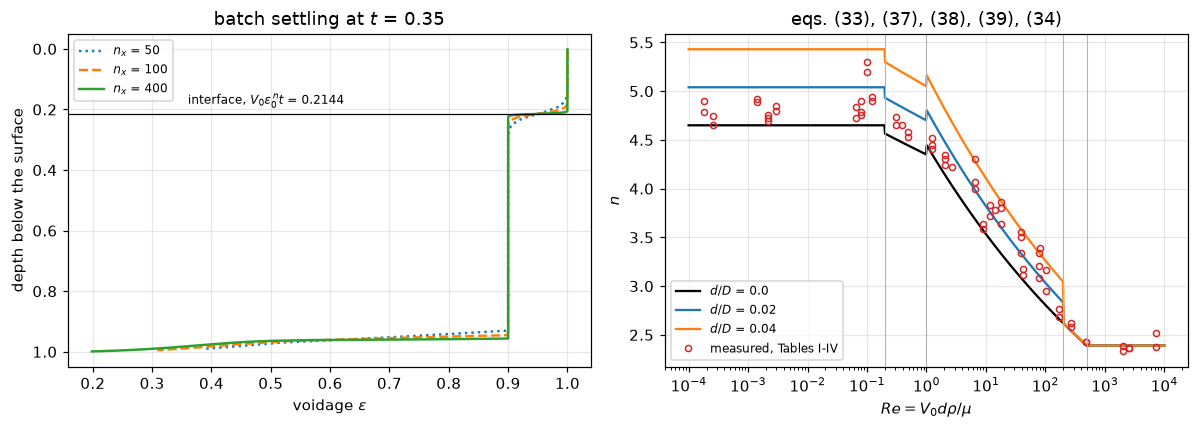
Richardson, J. F.; Zaki, W. N. (1954) — Transactions of the Institution of Chemical Engineers 32, 35-53 — table
      [ '32, 35-53' above is the CATALOGUE's page range, inherited and NOT verified: the reprint
        actually read numbers this paper S82-S100 and 35-53 appears nowhere on it. ]
# What a bed of a real particle from Table III does, run through the paper's own recipe.
def worked_example(flu, c=COEF, wall=1.0):
"""The paper's recipe on one Table III bed. ``wall`` is the coefficient of d/D in
log V0 - log Vi: 1 for fluidisation (eq. 41), 0 for sedimentation (eq. 40)."""
row = flu[(flu.particle == "Ballotini") & (flu.d_cm == 5.1e-2) & (flu.column_in == D_244_IN)].iloc[0]
n_row = float(n_rz(row.Re_printed, row.d_over_D_printed, c))
V_i = 10**(np.log10(row.V0_cm_s) - wall * row.d_over_D_printed)
return row, n_row, V_i, dict(worked_n_dev_pct=float(dev_pct(n_row, row.slope_n)),
worked_Vi_dev_pct=float(dev_pct(V_i, 10**row.intercept_log10_Vc_at_eps1)))
row, n_row, V_i, mWk = worked_example(flu)
print(f"Table III, {row.particle} d = {row.d_cm} cm in the {row.column_in} in. column")
print(f" printed Re = {row.Re_printed:g}, d/D = {row.d_over_D_printed:g}, V0 = {row.V0_cm_s} cm/s")
print(f" eq. (38) n = {n_row:.4f} against the measured slope {row.slope_n} "
f"({mWk['worked_n_dev_pct']:+.2f} %)")
print(f" eq. (41) V_i = {V_i:.4f} cm/s against the printed intercept "
f"10^{row.intercept_log10_Vc_at_eps1} = {10**row.intercept_log10_Vc_at_eps1:.4f} cm/s "
f"({mWk['worked_Vi_dev_pct']:+.2f} %)")
print(f" the velocity to hold this bed at eps = 0.6: V_c = V_i eps^n = "
f"{V_i*0.6**n_row:.4f} cm/s (measured n gives {10**row.intercept_log10_Vc_at_eps1*0.6**row.slope_n:.4f})")
claims.value("worked_n_dev_pct", mWk["worked_n_dev_pct"])
claims.value("worked_Vi_dev_pct", mWk["worked_Vi_dev_pct"])Table III, Ballotini d = 0.051 cm in the 2.44 in. column
printed Re = 41.72, d/D = 0.00823, V0 = 8.1 cm/s
eq. (38) n = 3.1663 against the measured slope 3.11 (+1.81 %)
eq. (41) V_i = 7.9479 cm/s against the printed intercept 10^0.91 = 8.1283 cm/s (-2.22 %)
the velocity to hold this bed at eps = 0.6: V_c = V_i eps^n = 1.5770 cm/s (measured n gives 1.6598)Validation
The pymrm solve: what it tests, and what it is blind to
The interface in a batch settler is a shock between \(\phi = 0\) above and \(\phi_0\) below. Its speed follows from Rankine-Hugoniot, \(F(\phi_0)/\phi_0\), which for this flux is \(V_0(1-\phi_0)^n\) identically, so comparing the two is algebra, not evidence, and the page says that where it prints the number.
The check that can fail is grid convergence of the whole profile against the exact shock solution, measured on a window well above the base so that the growing sediment (which the correlation was never measured for) does not enter. Successive observed orders are printed for the whole ladder, not only their mean.
def L1_error(x_c, phi, u_ref, phi0=PHI0):
    m = x_c < WINDOW
    exact = np.where(x_c[m] < u_ref * T_END, 0.0, phi0)
    return float(np.abs(phi[m] - exact).sum() * (x_c[1] - x_c[0]))


LADDER = [50, 100, 200, 400, 800, 1600]


def shock_study(nx=400, ladder=True, ref_u=None, **kw):
    """L1 error against the exact shock at ``nx`` cells, the successive orders over the
    mesh ladder and the solids balance. ``kw`` goes to :func:`settle`, so a defect is
    injected through the solver's own arguments or physical parameters."""
    n_, V0_, p0 = kw.get("n", N_REF), kw.get("V0", V0_REF), kw.get("phi0", PHI0)
    u_ref = V0_REF * (1.0 - PHI0)**N_REF if ref_u is None else ref_u
    xc, ph, bad = settle(nx, T_END, **kw)
    e = L1_error(xc, ph, u_ref, p0)
    solids = abs(ph.sum() * (H_REF / nx) - p0 * H_REF) / (p0 * H_REF)
    out = dict(pymrm_L1_nx400=e, pymrm_solids_residual=solids)
    errs, orders = [], []
    if ladder:
        for k in LADDER:
            xk, pk, _ = settle(k, T_END, **kw)
            errs.append(L1_error(xk, pk, u_ref, p0))
        orders = [float(np.log2(a / b)) for a, b in zip(errs[:-1], errs[1:])]
        out.update(pymrm_order_mean=float(np.mean(orders)), pymrm_order_min=min(orders),
                   pymrm_order_max=max(orders))
    return out, errs, orders


def ratio_study(nx=400, nx_ref=None):
    """Error of three defective runs relative to the clean run at ``nx_ref`` cells
    (the same grid as the defective runs unless a defect says otherwise)."""
    nx_ref = nx if nx_ref is None else nx_ref
    xr, pr, _ = settle(nx_ref, T_END)
    e_ref = L1_error(xr, pr, u_rz)
    own = V0_REF * (1.0 - PHI0)**3.0
    return dict(brk_nu1_ratio=L1_error(*settle(nx, T_END, nu=1)[:2], u_rz) / e_ref,
                brk_upwind_ratio=L1_error(*settle(nx, T_END, flip_upwind=True)[:2], u_rz) / e_ref,
                brk_n3_own_speed_ratio=L1_error(*settle(nx, T_END, n=3.0)[:2], own) / e_ref)


mS, errs, orders = shock_study()
print(f"L1 error against the exact shock solution on 0 < x < {WINDOW:g}")
for k, e, o in zip(LADDER, errs, [np.nan] + orders):
    print(f"  nx = {k:5d}   L1 = {e:.4e}" + ("" if np.isnan(o) else f"   order {o:.3f}"))
print(f"\nsuccessive orders {min(orders):.3f} to {max(orders):.3f}, mean {mS['pymrm_order_mean']:.3f}: "
      f"first-order upwind on a shock, whose error oscillates with where the shock sits in a cell.")
print(f"solids balance residual at nx = 400: {mS['pymrm_solids_residual']:.2e}")
claims.value("pymrm_L1_nx400", mS["pymrm_L1_nx400"])
claims.bound("pymrm_order_mean", mS["pymrm_order_mean"], min=0.9, max=1.1, basis="theory",
             note="first-order scheme on a shock")
claims.bound("pymrm_order_min", mS["pymrm_order_min"], min=0.8, max=1.2, basis="theory",
             note="successive orders oscillate with the shock's position in a cell")
claims.bound("pymrm_order_max", mS["pymrm_order_max"], min=0.8, max=1.2, basis="theory",
             note="successive orders oscillate with the shock's position in a cell")
claims.bound("pymrm_solids_residual", mS["pymrm_solids_residual"], max=1e-12, basis="identity",
             note="construct_div telescopes and both boundary fluxes are zero")
mRat = ratio_study()
for k in ("brk_nu1_ratio", "brk_upwind_ratio", "brk_n3_own_speed_ratio"):
    claims.value(k, mRat[k])
L1 error against the exact shock solution on 0 < x < 0.6
nx = 50 L1 = 1.7828e-03
nx = 100 L1 = 9.6647e-04 order 0.883
nx = 200 L1 = 4.4608e-04 order 1.115
nx = 400 L1 = 2.2646e-04 order 0.978
nx = 800 L1 = 1.2024e-04 order 0.913
nx = 1600 L1 = 5.5801e-05 order 1.108
successive orders 0.883 to 1.115, mean 1.000: first-order upwind on a shock, whose error oscillates with where the shock sits in a cell.
solids balance residual at nx = 400: 0.00e+00Break table: inject a defect, confirm the number moves
Every number above is registered as a claim; each row injects one defect through an argument of the function that computes the number, or through a constant or a data cell, and reports whether any claim’s own check catches it. The first row of each group is a control, the same computation with only the bootstrap stream changed: it must fail no claim. The two checks on trial in the pymrm solve are the L1 error against the exact shock and the global solids balance; the balance cannot fail for almost anything, and would have looked like the page’s cleanest result if quoted alone.
def coef_row(**kw):
    """A correlation with constants changed, and its label."""
    return dict(COEF, **kw), "; ".join(f"{k} = {v:g} instead of {COEF[k]:g}" for k, v in kw.items())


def corr_defect(A_x, c=COEF, edges=EDGES):
    """Everything section 2 and 4 report, evaluated with a defective correlation."""
    Ax = score_A(A_x, c, edges)
    kp = Ax[Ax.is_oil == 0]
    got = dict(section2_metrics(Ax))
    got["rz_windows"] = n_rz_windows(edges)
    got.update(eq37_study(kp, c)["metrics"])
    got.update(oil_metrics(Ax, edges))
    return got, kp


def row_for(label, got):
    brk_all(label, got)


# ---- transcription
for kw in [dict(g=9.81), dict(mu_unit=1.0), dict(cm_per_in=2.5)]:
    k, v = next(iter(kw.items()))
    row_for(f"{k} = {v:g} instead of {dict(g=G_CGS, mu_unit=1e-2, cm_per_in=CM_PER_IN)[k]:g}",
            transcription(sed, flu, **kw)["metrics"])
for df_name, col, fac, ridx in [("sed", "V0_cm_s", 1.1, 0), ("flu", "V0_cm_s", 1.1, 0),
                                ("flu", "d_over_D_printed", 0.9, 0)]:
    sx, fx = (perturbed(sed, col, fac, ridx), flu) if df_name == "sed" else (sed, perturbed(flu, col, fac, ridx))
    row_for(f"{df_name} row {ridx}: {col} x {fac:g}", transcription(sx, fx)["metrics"])
row_for("sed row 0: d_over_D_printed x 1.1 (one more cell off by more than 1 %)",
        transcription(perturbed(sed, "d_over_D_printed", 1.1, 0), flu)["metrics"])
row_for("every sedimentation row: d_cm x 0.998 (a bad cell would only join the listed anomalies)",
        transcription(sed.assign(d_cm=sed.d_cm * 0.998), flu)["metrics"])

# ---- the correlation (sections 2 and 4 share its constants)
row_for("control: no defect (correlation evaluated again)", corr_defect(build_A(sed, flu))[0])
for kw in [dict(a33=4.56), dict(a35=4.53), dict(a36=4.54), dict(p36=0.1), dict(s38=1.8), dict(s37=7.5),
           dict(n34=2.93)]:
    c, lab = coef_row(**kw)
    got, kp = corr_defect(build_A(sed, flu), c)
    row_for(lab, got)
    row_for(lab + " (section 4)", identities(n0t, c)["metrics"])
    if "p36" in kw:
        row_for(lab + " (residual correlations)", resid_metrics(kp, np.random.default_rng(7))["metrics"])
for edges, what in [((0.2, 1.0, 1.0, 500.0), "the Re = 200 window edge moved onto 1"),
                    ((0.1, 1.0, 200.0, 500.0), "the Re = 0.2 window edge moved to 0.1"),
                    ((0.2, 1.0, 200.0, 3000.0), "the Re = 500 window edge moved to 3000")]:
    got, _ = corr_defect(build_A(sed, flu), edges=edges)
    row_for(f"edges = {edges}: {what}", got)
got, _ = corr_defect(build_A(perturbed(sed, "slope_n", 10.0, 0), flu))
row_for("sed row 0: slope_n x 10 (decimal point lost)", got)
pos_hi = int(np.flatnonzero((flu.Re_printed > 500).values)[0])
got, _ = corr_defect(build_A(sed, perturbed(flu, "slope_n", 10.0, pos_hi)))
row_for(f"flu row {pos_hi} (Re above 500): slope_n x 10 (decimal point lost)", got)
got, _ = corr_defect(build_A(sed, flu).assign(is_oil=0))
row_for("oil flag lost on the oil rows", got)
got, _ = corr_defect(build_A(sed[sed.table == "I"], flu))
row_for("Table II not read", got)
row_for("control: residual correlations, other cluster seed",
        resid_metrics(keep, np.random.default_rng(7))["metrics"])
row_for("residual intervals with every row its own cluster",
        resid_metrics(keep, np.random.default_rng(7), cluster="row")["metrics"])

# ---- identities of section 4 on the data
top_pos = int(np.argmax(n0t.Re.values))
for col, fac, ridx in [("Re", 498 / 489, top_pos), ("n0_printed", 1.1, top_pos),
                       ("slope_n_vs_dD_printed", 1.1, 0), ("minus_dD_at_n0_printed", 2.0, 0)]:
    row_for(f"Table VI/VII row {ridx}: {col} x {fac:.4g}", identities(perturbed(n0t, col, fac, ridx))["metrics"])

# ---- non-spherical particles
for kw in [dict(slope_col="slope_15"), dict(k_power=2)]:
    k, v = next(iter(kw.items()))
    row_for(f"nonspherical({k}={v!r}) instead of {dict(slope_col='slope_244', k_power=3)[k]!r}",
            nonspherical(nsp, **kw)["metrics"])
for kw in [dict(a42=2.07), dict(p42=0.61), dict(n34=2.93)]:
    c, lab = coef_row(**kw)
    row_for(lab, nonspherical(nsp, c)["metrics"])
pos_cyl = int(np.flatnonzero((nsp.particle == "Steel cylinder").values)[0])
row_for("Table VIII row 0: n_table8 x 1.1",
        nonspherical(perturbed(nsp, "n_table8", 1.1, 0))["metrics"])
row_for(f"Table V row {pos_cyl} (Steel cylinder): d_s_cm x 1.1",
        nonspherical(perturbed(nsp, "d_s_cm", 1.1, pos_cyl))["metrics"])

# ---- worked example
c_, lab = coef_row(a36=4.54)
row_for(lab, worked_example(flu, c_)[3])
row_for("sedimentation wall law (eq. 40) used for a fluidised bed: wall = 0", worked_example(flu, wall=0.0)[3])

# ---- wall laws
def shifted(df, delta, column_in=None):
    out = df.copy()
    sel = np.ones(len(out), bool) if column_in is None else (out.column_in == column_in).values
    out.loc[sel, "intercept_log10_Vc_at_eps1"] += delta
    return out


def swapped(df):
    """Copy with the two columns of y = log10 V0 - intercept exchanged (alpha changes sign)."""
    return df.assign(log10_V0_printed=df.intercept_log10_Vc_at_eps1,
                     intercept_log10_Vc_at_eps1=df.log10_V0_printed)


row_for("intercept column read 0.03 decades high on every row",
        wall_study(shifted(sed, 0.03), shifted(flu, 0.03), np.random.default_rng(7))["metrics"])
row_for("log10 V0 and intercept columns exchanged (y with the wrong sign)",
        wall_study(swapped(sed), swapped(flu), np.random.default_rng(7))["metrics"])
row_for("wall intervals with every row its own cluster",
        wall_study(sed, flu, np.random.default_rng(7), cluster="row")["metrics"])
row_for("paired test: 2.44 in. column intercepts read 0.02 decades high",
        paired_study(shifted(flu, 0.02, D_244_IN))["metrics"])
row_for("paired test: resolution of a difference taken as 0.05 instead of 0.01",
        paired_study(flu, quant=0.05)["metrics"])
row_for("paired test: lead shot pairs missing",
        paired_study(flu[flu.particle != "Lead shot"])["metrics"])

# ---- the pymrm solve
row_for("control: shock ladder unchanged", shock_study(ladder=False)[0])
for kw in [dict(nu=1), dict(sign=-1.0), dict(flip_upwind=True), dict(cfl=1.6), dict(n=3.0), dict(V0=1.01)]:
    k, v = next(iter(kw.items()))
    lab = f"settle({k}={v!r}) instead of {dict(nu=0, sign=1.0, flip_upwind=False, cfl=0.4, n=N_REF, V0=V0_REF)[k]!r}"
    row_for(lab, shock_study(ladder=False, **kw)[0])
row_for(f"settle(n=3.0) judged against its own shock speed",
        shock_study(ladder=False, n=3.0, ref_u=V0_REF * (1.0 - PHI0)**3.0)[0])
row_for("mesh: nx = 25 instead of 400", shock_study(nx=25, ladder=False)[0])
for kw in [dict(nu=1), dict(flip_upwind=True)]:
    k, v = next(iter(kw.items()))
    row_for(f"mesh ladder with settle({k}={v!r})", shock_study(**kw)[0])
row_for("ratios against a clean run at nx = 50 instead of nx = 400", ratio_study(nx_ref=50))
# The break table, after every claim is registered: one line per row, with the claims it fails.
by_row = {}
for r_, m_, clean_, broken_, caught_ in BREAK:
by_row.setdefault(r_, []).append((m_, caught_))
controls = [r_ for r_ in by_row if r_.startswith("control")]
_bad = [(r_, m_, f"{c0:.4g}", f"{b:.4g}") for r_, m_, c0, b, c_ in BREAK if c_ and r_ in controls]
assert not _bad, f"a control row failed a claim: {_bad}"
print(f"{'injected defect':<88} {'claims failed':>13} of {'reported':>8}")
for r_, ms in by_row.items():
print(f"{r_[:88]:<88} {sum(c_ for _, c_ in ms):13d} of {len(ms):8d}")
_caught = {m_ for _, m_, _, _, c_ in BREAK if c_}
_open = sorted(k for k in claims.metrics if k not in _caught and not claims.metrics[k].get("structural"))
print(f"\n{len(by_row)} rows ({len(controls)} controls, which fail no claim); "
f"{len(_caught)} of {len(claims.metrics)} claims are failed by at least one row; "
f"open: {', '.join(_open) or 'none'}")injected defect claims failed of reported
g = 9.81 instead of 981 3 of 11
mu_unit = 1 instead of 0.01 6 of 11
cm_per_in = 2.5 instead of 2.54 2 of 11
sed row 0: V0_cm_s x 1.1 4 of 11
flu row 0: V0_cm_s x 1.1 3 of 11
flu row 0: d_over_D_printed x 0.9 1 of 11
sed row 0: d_over_D_printed x 1.1 (one more cell off by more than 1 %) 1 of 11
every sedimentation row: d_cm x 0.998 (a bad cell would only join the listed anomalies) 3 of 11
control: no defect (correlation evaluated again) 0 of 28
a33 = 4.56 instead of 4.65 3 of 28
a33 = 4.56 instead of 4.65 (section 4) 3 of 14
a35 = 4.53 instead of 4.35 7 of 28
a35 = 4.53 instead of 4.35 (section 4) 3 of 14
a36 = 4.54 instead of 4.45 9 of 30
a36 = 4.54 instead of 4.45 (section 4) 5 of 14
p36 = 0.1 instead of -0.1 8 of 28
p36 = 0.1 instead of -0.1 (section 4) 3 of 14
p36 = 0.1 instead of -0.1 (residual correlations) 3 of 4
s38 = 1.8 instead of 18 8 of 28
s38 = 1.8 instead of 18 (section 4) 3 of 14
s37 = 7.5 instead of 17.5 7 of 28
s37 = 7.5 instead of 17.5 (section 4) 1 of 14
n34 = 2.93 instead of 2.39 4 of 37
n34 = 2.93 instead of 2.39 (section 4) 1 of 14
edges = (0.2, 1.0, 1.0, 500.0): the Re = 200 window edge moved onto 1 9 of 28
edges = (0.1, 1.0, 200.0, 500.0): the Re = 0.2 window edge moved to 0.1 7 of 28
edges = (0.2, 1.0, 200.0, 3000.0): the Re = 500 window edge moved to 3000 3 of 28
sed row 0: slope_n x 10 (decimal point lost) 7 of 28
flu row 0 (Re above 500): slope_n x 10 (decimal point lost) 6 of 28
oil flag lost on the oil rows 12 of 28
Table II not read 6 of 28
control: residual correlations, other cluster seed 0 of 4
residual intervals with every row its own cluster 1 of 4
Table VI/VII row 18: Re x 1.018 2 of 14
Table VI/VII row 18: n0_printed x 1.1 2 of 14
Table VI/VII row 0: slope_n_vs_dD_printed x 1.1 2 of 14
Table VI/VII row 0: minus_dD_at_n0_printed x 2 3 of 14
nonspherical(slope_col='slope_15') instead of 'slope_244' 1 of 9
nonspherical(k_power=2) instead of 3 2 of 9
a42 = 2.07 instead of 2.7 3 of 9
p42 = 0.61 instead of 0.16 3 of 9
Table VIII row 0: n_table8 x 1.1 5 of 9
Table V row 4 (Steel cylinder): d_s_cm x 1.1 1 of 9
sedimentation wall law (eq. 40) used for a fluidised bed: wall = 0 1 of 2
intercept column read 0.03 decades high on every row 28 of 31
log10 V0 and intercept columns exchanged (y with the wrong sign) 27 of 31
wall intervals with every row its own cluster 12 of 31
paired test: 2.44 in. column intercepts read 0.02 decades high 3 of 5
paired test: resolution of a difference taken as 0.05 instead of 0.01 4 of 5
paired test: lead shot pairs missing 1 of 5
control: shock ladder unchanged 0 of 2
settle(nu=1) instead of 0 2 of 2
settle(sign=-1.0) instead of 1.0 1 of 2
settle(flip_upwind=True) instead of False 1 of 2
settle(cfl=1.6) instead of 0.4 1 of 2
settle(n=3.0) instead of 4.65 1 of 2
settle(V0=1.01) instead of 1.0 1 of 2
settle(n=3.0) judged against its own shock speed 1 of 2
mesh: nx = 25 instead of 400 1 of 2
mesh ladder with settle(nu=1) 5 of 5
mesh ladder with settle(flip_upwind=True) 4 of 5
ratios against a clean run at nx = 50 instead of nx = 400 3 of 3
62 rows (3 controls, which fail no claim); 112 of 112 claims are failed by at least one row; open: noneWhat the solve and its break rows say
_solids = [(r_, c_, b) for r_, m_, c0, b, c_ in BREAK if m_ == "pymrm_solids_residual" and not r_.startswith("control")]
nu1 = next(b for r_, c_, b in _solids if r_.startswith("settle(nu=1)"))
other_zero = [r_ for r_, c_, b in _solids if not c_]
display(Markdown(
    f"**The solids balance is a check that rarely fails.** It stays at round-off for "
    f"{len(other_zero)} of the {len(_solids)} injected defects that report it, "
    f"including a flipped flux sign, a reversed upwind direction, a wrong exponent, a wrong $V_0$, "
    f"an unstable time step and a 25-cell grid. That is structural: `construct_div` telescopes, "
    f"and both boundary fluxes are set to zero, so the total is conserved whatever is put into "
    f"the interior faces. The only defect it catches is `nu = 1` ({nu1:.2f}), because a cylindrical "
    f"divergence does not telescope on a Cartesian grid. Quoting the balance residual as evidence "
    f"that the settling model is right would be exactly the defect the verifier brief exists to "
    f"catch.\n\n"
    f"**The L1 error is a real check on the discretisation and on nothing else.** "
    f"It moves by {mRat['brk_nu1_ratio']:.0f}x for `nu = 1` and "
    f"{mRat['brk_upwind_ratio']:.0f}x for a reversed upwind direction. But set $n = 3.00$ and judge "
    f"the result against the shock speed *that value of $n$ implies* and the "
    f"error moves by only {mRat['brk_n3_own_speed_ratio']:.1f}x, **the solve "
    f"has no opinion about the value of $n$ at all.** A 1 % error in $V_0$ is "
    f"likewise almost invisible, because a 1 % shift of the interface is "
    f"comparable to the width the first-order scheme smears it over. Nothing in "
    f"this section is evidence for or against Richardson and Zaki's correlation; "
    f"it is evidence that the flux was integrated correctly."))
The solids balance is a check that rarely fails. It stays at round-off for 8 of the 10 injected defects that report it, including a flipped flux sign, a reversed upwind direction, a wrong exponent, a wrong \(V_0\), an unstable time step and a 25-cell grid. That is structural: construct_div telescopes, and both boundary fluxes are set to zero, so the total is conserved whatever is put into the interior faces. The only defect it catches is nu = 1 (0.37), because a cylindrical divergence does not telescope on a Cartesian grid. Quoting the balance residual as evidence that the settling model is right would be exactly the defect the verifier brief exists to catch.
The L1 error is a real check on the discretisation and on nothing else. It moves by 111x for nu = 1 and 187x for a reversed upwind direction. But set \(n = 3.00\) and judge the result against the shock speed that value of \(n\) implies and the error moves by only 1.5x, the solve has no opinion about the value of \(n\) at all. A 1 % error in \(V_0\) is likewise almost invisible, because a 1 % shift of the interface is comparable to the width the first-order scheme smears it over. Nothing in this section is evidence for or against Richardson and Zaki’s correlation; it is evidence that the flux was integrated correctly.
Every agreement number on this page, and whether it can fail
| what is compared | where | can it fail? |
|---|---|---|
| the printed identities against the transcription | §1 | yes, on the named cells |
| Stokes’ law against Table I, and against Table II | §1 | yes, and it must fail on Table II, it does |
| eqs. (33)-(39) against the non-oil measured slopes | §2 | yes, but it is a fit residual: these are the data the fit was made on |
| constant-\(n\) null baseline per branch | §2 | it is the baseline; eq. (34) coincides with it |
| eq. (37) against its null | §2 | no, it decides nothing: the gap reverses under two sensitivities and splits under the third |
| residual against \(\mu\), \(\rho\), \(\rho_s/\rho\) | §2 | yes, a null result, cluster-bootstrapped |
| wall coefficient \(\alpha\), sedimentation vs fluidisation | §3 | yes, on Table I and on Tables III+IV: each law is falsifiable on the other’s data |
| the Table II rows inside the pooled fit | §3 | no: their residual is zero to the printed digits because the intercept column reproduces \(\log_{10}V_0\); excluded from the headline |
| paired wall test across the two columns | §3 | yes, on the pairs above the printed resolution; the others cannot resolve it |
| Table VI \(\times\) Table VII transformation | §4 | yes: any transcription slip breaks it |
| eq. (39) at \(Re = 500\) against eq. (34) | §4 | as a transcription check, yes; as evidence of two independent fits, no: Table VI’s last row is eq. (34)’s constant |
| eqs. (35)/(36) against Table VI | §4 | fit residual |
| eq. (42) against Table VIII, with a null | §5 | yes, and the null nearly matches it |
| \(K\) recomputed from printed \(d_s\), \(d_p\) | §5 | yes: it fails on some rows |
| pymrm \(L1\) against the exact shock | Validation | yes: successive orders, break rows |
| pymrm solids balance | Validation | almost never: structural, and the break rows show which defect it does catch |
| RH speed against \(V_0\varepsilon_0^n\) | Validation | no: algebraically identical, and said so |
| the correlation’s constants and window edges, via the crossovers and coefficient checks | §4 | yes: every constant has a break row |
What pymrm adds
def fill(text, **kw):
    """Put computed numbers into prose: ``@@name@@`` is replaced by ``kw['name']``."""
    for k, v in kw.items():
        text = text.replace(f"@@{k}@@", str(v))
    return text


display(Markdown(fill(r"""**To the correlation: nothing.** Equations (33)-(42) are algebra and need no
solver, and this page does not pretend otherwise. What the reimplementation adds
is the following, none of which is a differential equation.

**The tables, machine-readable, with the transcription certified by identities
the paper itself prints.** What is usually cited of Richardson and Zaki is one
line of it. The @@ncmp@@ measured exponents, the @@nn0@@ $n_0$
values and the two intercept columns are here as
four CSVs, and the identities of §1 say how far they
can be trusted, including the places where the printing is wrong.

**The correlation costed against a null model, window by window.** The
whole-table agreement of @@mad@@ % is not the useful number. Of the five printed
expressions, eq. (38) beats a constant by a factor of @@fac38@@ on @@n38@@
rows, eq. (33) beats it modestly, eq. (34) *is* a constant, and **eq. (37) is not
distinguishable from a constant in either direction on the @@n37@@ rows that fall in
its window**: the @@gap37@@-percentage-point gap between them reverses if the two
rows of disputed branch are moved and if the in-sample null is charged for the
parameter it fits, and splits under leave-one-out (the correlation is ahead in
@@loo@@ of @@n37@@ deletions). That statement is not in the paper and it is the one a
reader needs before trusting the $0.2 < Re < 1$ branch.

**The two wall laws decided on the authors' own numbers, on the rows that could
have decided otherwise.** Fitting the single coefficient $\alpha$ in
$\log V_0 - \log V_i = \alpha(d/D)$ separately to the sedimentation and
fluidisation tables gives intervals that exclude each other and that pick, in
each case, the equation the authors applied there. This is the page's strongest
result and its limits are stated: **Table II's intercept column reproduces its
own $\log_{10} V_0$ column on all @@n2@@ rows**, @@nz@@ of them to the printed three
decimals and the remaining one being the same number with its minus sign lost, so
@@nz@@ of the @@nsed@@ sedimentation rows in the fit carry a residual of zero to the printed digits and cannot
detect a wall effect of any size. The sedimentation fit is therefore quoted on
Table I alone, at the @@narrow@@-times-wider interval §3 prints, and the verdict is
unchanged. The fluidisation number is a refit of the data Fig. 21 was drawn from;
the sedimentation number is not. And on the $d/D$ range the two data sets share,
the fluidisation interval **excludes** eq. (41)'s coefficient of 1: $\alpha$ is
@@alo@@ below $d/D = 0.05$ and @@ahi@@ above it, so the *linear* form of
eq. (41) does not hold across its own range even though the two-law verdict does.
All of these numbers are printed in §3.

**Three arithmetic findings, all small and all worth knowing.** The 17.5 and 18
of eqs. (37) and (38) are @@e175@@ and @@e18@@ rounded up, from the division displayed
on the line above them. The mean of Table VII is @@mdd@@, not the 0.25 the text
quotes. And the branch boundary at $Re = 200$ is discontinuous by @@j200@@ % in
$n$ at $d/D = 0.04$ because eq. (39) drops the wall term, which anyone sweeping
$Re$ through 200 in a solver will meet, and which is invisible at $d/D = 0$ where
it is usually plotted.

**The flux function integrated, with the honest accounting of what that shows.**
$F(\phi) = \phi V_0(1-\phi)^n$ is what the correlation becomes downstream, in
every thickener and batch-settling model. The pymrm solve converges at order about 1 on
the interface and its global solids balance is at round-off, and the break
table shows that the balance is at round-off for a wrong $n$, a wrong $V_0$, an
unstable step and a coarse grid as well. The solve tests the integration, not the
physics, and the page states that rather than banking the round-off.""",
    ncmp=claims["n_comparisons"], nn0=int(n0t.n0_printed.notna().sum()), mad=f"{claims['corr_nonoil_mean_abs_pct']:.1f}",
    fac38=f"{r38_null/r38_rz:.1f}", n38=len(b38), n37=len(b37),
    gap37=f"{abs(r37_rz - r37_null):.2f}", loo=n_flip, n2=len(tII_all), nz=n_zero_rows, nsed=len(sed_fit),
    narrow=f"{claims['wall_pooled_ci_narrowing']:.0f}",
    alo=f"{claims['wall_alpha_flu_dD_below_005']:.1f}", ahi=f"{claims['wall_alpha_flu_dD_above_005']:.1f}",
    e175=f"{I4['exact175']:.1f}", e18=f"{I4['exact18']:.1f}", mdd=f"{claims['tableVII_mean_dD']:.4f}",
    j200=f"{abs(claims['crossover_Re200_dD004_pct']):.0f}")))
To the correlation: nothing. Equations (33)-(42) are algebra and need no solver, and this page does not pretend otherwise. What the reimplementation adds is the following, none of which is a differential equation.
The tables, machine-readable, with the transcription certified by identities the paper itself prints. What is usually cited of Richardson and Zaki is one line of it. The 66 measured exponents, the 18 \(n_0\) values and the two intercept columns are here as four CSVs, and the identities of §1 say how far they can be trusted, including the places where the printing is wrong.
The correlation costed against a null model, window by window. The whole-table agreement of 1.2 % is not the useful number. Of the five printed expressions, eq. (38) beats a constant by a factor of 7.5 on 23 rows, eq. (33) beats it modestly, eq. (34) is a constant, and eq. (37) is not distinguishable from a constant in either direction on the 5 rows that fall in its window: the 0.02-percentage-point gap between them reverses if the two rows of disputed branch are moved and if the in-sample null is charged for the parameter it fits, and splits under leave-one-out (the correlation is ahead in 2 of 5 deletions). That statement is not in the paper and it is the one a reader needs before trusting the \(0.2 < Re < 1\) branch.
The two wall laws decided on the authors’ own numbers, on the rows that could have decided otherwise. Fitting the single coefficient \(\alpha\) in \(\log V_0 - \log V_i = \alpha(d/D)\) separately to the sedimentation and fluidisation tables gives intervals that exclude each other and that pick, in each case, the equation the authors applied there. This is the page’s strongest result and its limits are stated: Table II’s intercept column reproduces its own \(\log_{10} V_0\) column on all 15 rows, 14 of them to the printed three decimals and the remaining one being the same number with its minus sign lost, so 14 of the 36 sedimentation rows in the fit carry a residual of zero to the printed digits and cannot detect a wall effect of any size. The sedimentation fit is therefore quoted on Table I alone, at the 4-times-wider interval §3 prints, and the verdict is unchanged. The fluidisation number is a refit of the data Fig. 21 was drawn from; the sedimentation number is not. And on the \(d/D\) range the two data sets share, the fluidisation interval excludes eq. (41)’s coefficient of 1: \(\alpha\) is 2.2 below \(d/D = 0.05\) and 1.0 above it, so the linear form of eq. (41) does not hold across its own range even though the two-law verdict does. All of these numbers are printed in §3.
Three arithmetic findings, all small and all worth knowing. The 17.5 and 18 of eqs. (37) and (38) are 17.4 and 17.8 rounded up, from the division displayed on the line above them. The mean of Table VII is 0.2457, not the 0.25 the text quotes. And the branch boundary at \(Re = 200\) is discontinuous by 14 % in \(n\) at \(d/D = 0.04\) because eq. (39) drops the wall term, which anyone sweeping \(Re\) through 200 in a solver will meet, and which is invisible at \(d/D = 0\) where it is usually plotted.
The flux function integrated, with the honest accounting of what that shows. \(F(\phi) = \phi V_0(1-\phi)^n\) is what the correlation becomes downstream, in every thickener and batch-settling model. The pymrm solve converges at order about 1 on the interface and its global solids balance is at round-off, and the break table shows that the balance is at round-off for a wrong \(n\), a wrong \(V_0\), an unstable step and a coarse grid as well. The solve tests the integration, not the physics, and the page states that rather than banking the round-off.
What this page does not claim
display(Markdown(fill(r"""**It is not experimentally validated.** The data are the authors' own
measurements, so the *data tier* is 2, but eqs. (33)-(39) were fitted to these
very slopes, and the @@mad@@ % is a fit residual. There is no hold-out set. The only
rows the authors excluded, the two oils at high $d/D$, are excluded for a reason
that is perfectly confounded with the correlation's own stated $d/D$ limit, so
they cannot serve as one either.

**It says nothing about $\varepsilon$ outside roughly 0.42 to 0.96.** Equation
(28) is a straight line on $\log V_c$ against $\log\varepsilon$ over whatever
range each run covered, and the tables record only its slope and intercept. The
most extreme printed abscissa tick this page read on any of those figures is
$\log\varepsilon = -0.38$ (Fig. 12, $\varepsilon = 0.42$), the least extreme
$-0.02$ ($\varepsilon = 0.96$); those are **printed axis labels, not digitised
coordinates**, and no point was read off any figure. Everything the pymrm section
does below that voidage, which is the whole basal sediment, is outside the
correlation's measured range and is labelled so.

**It says nothing about non-uniform or non-spherical suspensions beyond
Table VIII.** The paper's own summary is explicit: "The present study has been
confined to relatively large particles ($d > 100$ microns)"; "The sedimentation
tests have all been carried out with uniform particles". Its mixed-size result is
a single figure (Fig. 15) with no tabulated numbers, and this page does not
reproduce it.

**The wall verdict is about $\alpha$, not about the mechanism.** The fits show a
$d/D$ term in the fluidisation intercepts and none in the sedimentation
intercepts. That the difference is "a velocity gradient created in the liquid
because of the drag exerted by the walls" is the authors' explanation, and
nothing in the tables tests it.

**And it is about the *presence* of the term, not the coefficient 1.** The
sedimentation half of that verdict rests on Table I alone, because Table II's
intercept column reproduces its own $\log_{10} V_0$ column and its @@nz@@ rows
in the fit cannot show a wall effect of any size; the interval on Table I is wide,
and it is the one quoted. The fluidisation half is a refit of the figure eq. (41)
was read off, and on the $d/D$ range the two data sets share it excludes 1 rather
than containing it. The page claims a wall term in fluidisation and none in
sedimentation. It does not claim that $\log V_0 - \log V_i$ equals $d/D$.

**The eq. (37) branch is not adjudicated.** Its rows cannot separate the
correlation from a constant, in either direction, and §2 prints the three
sensitivities that show why. Nothing on this page says eq. (37) is worse than a
constant.

**Table V's $d_s$ column is illegible in this scan** and no result on this page
depends on it. That is why §5's $K$ finding is stated as "eq. (42)'s abscissa
cannot be reconstructed for @@nbad@@ of its @@nx@@ points" rather than as "the
printed $K$ is wrong".

**Three quantities used here are not printed in the paper.** Water at 20 °C
($\mu = 1$ cP, $\rho = 1$), used only to re-check Table III's $Re$ column; the
two column diameters in cm, fixed to below 0.3 % by the printed $d/D$ column; and
$g = 981$ cm s$^{-2}$, used only for Stokes' law in §1. None enters a result.

**The batch-settling balance is not Richardson and Zaki's.** They write no
conservation law. The balance in the pymrm section is derived on the page from a
solids volume balance; the kinematic-wave treatment of batch sedimentation is
standard and older than this paper, and no specific source is cited for it
because none was consulted. What is theirs is $F(\phi)$.

**No figure was digitised, and no claim here rests on one.** The only
figure-derived quantities anywhere on the page are printed axis tick labels,
quoted as printed text.""", mad=f"{claims['corr_nonoil_mean_abs_pct']:.1f}", nz=n_zero_rows,
    nbad=len(bad), nx=len(x))))
It is not experimentally validated. The data are the authors’ own measurements, so the data tier is 2, but eqs. (33)-(39) were fitted to these very slopes, and the 1.2 % is a fit residual. There is no hold-out set. The only rows the authors excluded, the two oils at high \(d/D\), are excluded for a reason that is perfectly confounded with the correlation’s own stated \(d/D\) limit, so they cannot serve as one either.
It says nothing about \(\varepsilon\) outside roughly 0.42 to 0.96. Equation (28) is a straight line on \(\log V_c\) against \(\log\varepsilon\) over whatever range each run covered, and the tables record only its slope and intercept. The most extreme printed abscissa tick this page read on any of those figures is \(\log\varepsilon = -0.38\) (Fig. 12, \(\varepsilon = 0.42\)), the least extreme \(-0.02\) (\(\varepsilon = 0.96\)); those are printed axis labels, not digitised coordinates, and no point was read off any figure. Everything the pymrm section does below that voidage, which is the whole basal sediment, is outside the correlation’s measured range and is labelled so.
It says nothing about non-uniform or non-spherical suspensions beyond Table VIII. The paper’s own summary is explicit: “The present study has been confined to relatively large particles (\(d > 100\) microns)”; “The sedimentation tests have all been carried out with uniform particles”. Its mixed-size result is a single figure (Fig. 15) with no tabulated numbers, and this page does not reproduce it.
The wall verdict is about \(\alpha\), not about the mechanism. The fits show a \(d/D\) term in the fluidisation intercepts and none in the sedimentation intercepts. That the difference is “a velocity gradient created in the liquid because of the drag exerted by the walls” is the authors’ explanation, and nothing in the tables tests it.
And it is about the presence of the term, not the coefficient 1. The sedimentation half of that verdict rests on Table I alone, because Table II’s intercept column reproduces its own \(\log_{10} V_0\) column and its 14 rows in the fit cannot show a wall effect of any size; the interval on Table I is wide, and it is the one quoted. The fluidisation half is a refit of the figure eq. (41) was read off, and on the \(d/D\) range the two data sets share it excludes 1 rather than containing it. The page claims a wall term in fluidisation and none in sedimentation. It does not claim that \(\log V_0 - \log V_i\) equals \(d/D\).
The eq. (37) branch is not adjudicated. Its rows cannot separate the correlation from a constant, in either direction, and §2 prints the three sensitivities that show why. Nothing on this page says eq. (37) is worse than a constant.
Table V’s \(d_s\) column is illegible in this scan and no result on this page depends on it. That is why §5’s \(K\) finding is stated as “eq. (42)’s abscissa cannot be reconstructed for 4 of its 7 points” rather than as “the printed \(K\) is wrong”.
Three quantities used here are not printed in the paper. Water at 20 °C (\(\mu = 1\) cP, \(\rho = 1\)), used only to re-check Table III’s \(Re\) column; the two column diameters in cm, fixed to below 0.3 % by the printed \(d/D\) column; and \(g = 981\) cm s\(^{-2}\), used only for Stokes’ law in §1. None enters a result.
The batch-settling balance is not Richardson and Zaki’s. They write no conservation law. The balance in the pymrm section is derived on the page from a solids volume balance; the kinematic-wave treatment of batch sedimentation is standard and older than this paper, and no specific source is cited for it because none was consulted. What is theirs is \(F(\phi)\).
No figure was digitised, and no claim here rests on one. The only figure-derived quantities anywhere on the page are printed axis tick labels, quoted as printed text.
Reuse
# The correlation, as printed.  Re is built on the TERMINAL velocity, so n is a
# property of the particle/liquid/tube combination and does not move with u.
def n_richardson_zaki(Re, dD):
    if Re <= 0.2:  return 4.65 + 19.5 * dD                    # eq. (33)
    if Re <= 1.0:  return (4.35 + 17.5 * dD) * Re**-0.03      # eq. (37)
    if Re <= 200:  return (4.45 + 18.0 * dD) * Re**-0.1       # eq. (38)
    if Re <= 500:  return 4.45 * Re**-0.1                     # eq. (39)
    return 2.39                                               # eq. (34)

# The authors' own recipe, page S97.  Do NOT drop the wall term in fluidisation.
V_i = V_0                              if sedimentation else V_0 * 10**(-d / D)   # eqs. (40), (41)
n   = n_richardson_zaki(V_0 * d * rho / mu, d / D)
V_c = V_i * eps**n                                                                # eq. (28)

# As a flux, which is what downstream models want:
F = lambda phi: phi * V_0 * (1.0 - phi)**ndisplay(Markdown(fill(r"""**Three things to check before carrying this anywhere.**
1. **Which velocity you have.** The famous $u/u_t = \varepsilon^n$ is eq. (28)
with $V_i$ replaced by $V_0$, i.e. eq. (40). In a column with $d/D = 0.04$ the
wall term of eq. (41) is a factor $10^{-0.04} = @@fw@@$, a @@pw@@ % error, larger
than the worst deviation of the correlation from its own data on this page
(@@mx@@ %).
2. **Where your $Re$ sits.** At $Re = 200$ the index jumps by up to @@j200@@ % because
eq. (39) has no $d/D$ in it. At $Re = 0.2$ and $Re = 1$ there are smaller
jumps. If you are sweeping $Re$, smooth the branches or expect kinks.
3. **How far outside $d/D \le 0.04$ you are.** That is the authors' stated limit
and the only rows in the tables that exceed it inside the eq. (38) window are
the ones the authors themselves discard.
**Where this connects in the gallery.**
- [`A1.1`](../A1.1-ergun-pressure-drop/): Ergun. The fixed-bed end of the same
$\varepsilon(u)$ curve; the bed stops obeying Ergun and starts obeying
Richardson-Zaki at minimum fluidisation.
- `A1.6`: Wen and Yu's minimum fluidisation velocity. The other end of the
matching condition, and **not built here**.
- [`A1.7`](../A1.7-geldart-classification/): Geldart. Decides which fluidised-bed
model applies at all; its group A is defined by *smooth expansion before
bubbling*, which is the regime this correlation describes.
- `E1.1`: the two-phase theory. The gas-solid analogue of the expansion
question; parked, see its case file.
**What to change first if you reuse this.** $V_0$. Every branch boundary and
every wall correction is computed from it, and the paper obtains it either by
measurement or from published drag data it does not reproduce. An error in
$V_0$ moves $Re$ by the same fraction, which is enough to cross a branch boundary
for a particle whose $Re$ sits near 1, 200 or 500.""",
fw=f"{10**-0.04:.3f}", pw=f"{(1 - 10**-0.04) * 100:.0f}", mx=f"{claims['corr_nonoil_max_abs_pct']:.1f}",
j200=f"{abs(claims['crossover_Re200_dD004_pct']):.0f}")))Three things to check before carrying this anywhere.
- Which velocity you have. The famous \(u/u_t = \varepsilon^n\) is eq. (28) with \(V_i\) replaced by \(V_0\), i.e. eq. (40). In a column with \(d/D = 0.04\) the wall term of eq. (41) is a factor \(10^{-0.04} = 0.912\), a 9 % error, larger than the worst deviation of the correlation from its own data on this page (6.8 %).
- Where your \(Re\) sits. At \(Re = 200\) the index jumps by up to 14 % because eq. (39) has no \(d/D\) in it. At \(Re = 0.2\) and \(Re = 1\) there are smaller jumps. If you are sweeping \(Re\), smooth the branches or expect kinks.
- How far outside \(d/D \le 0.04\) you are. That is the authors’ stated limit and the only rows in the tables that exceed it inside the eq. (38) window are the ones the authors themselves discard.
Where this connects in the gallery.
A1.1: Ergun. The fixed-bed end of the same \(\varepsilon(u)\) curve; the bed stops obeying Ergun and starts obeying Richardson-Zaki at minimum fluidisation.A1.6: Wen and Yu’s minimum fluidisation velocity. The other end of the matching condition, and not built here.A1.7: Geldart. Decides which fluidised-bed model applies at all; its group A is defined by smooth expansion before bubbling, which is the regime this correlation describes.E1.1: the two-phase theory. The gas-solid analogue of the expansion question; parked, see its case file.
What to change first if you reuse this. \(V_0\). Every branch boundary and every wall correction is computed from it, and the paper obtains it either by measurement or from published drag data it does not reproduce. An error in \(V_0\) moves \(Re\) by the same fraction, which is enough to cross a branch boundary for a particle whose \(Re\) sits near 1, 200 or 500.
# Claims: prints every registered number, writes agreement.json for CI, and
# raises when a claim fails its own check or has no break row.
claims.report();   # the semicolon keeps the notebook from echoing the payload
Claims for A1.5:
transcription_dD_max_pct = 0.78261 value rtol 0.05
tableIII_dD_max_pct = 0.21429 value rtol 0.05
transcription_Re_max_pct = 3.7968 value rtol 0.05
Re_rows_above_half_pct = 4 exact exact, margin 0.115
printed_errors_listed = 6 exact exact, margin 0.217
transcription_logV0_max_decades = 0.010713 value rtol 0.05
stokes_tableI_max_pct = 0.67301 value rtol 0.05
stokes_tableII_settling_min_pct = 19.463 value rtol 0.05
stokes_tableII_settling_max_pct = 65.787 value rtol 0.05
column_244_in_cm = 6.1976 value rtol 1e-09
column_15_in_cm = 3.81 value rtol 1e-09
n_comparisons = 66 exact exact
n_rows_nonoil = 58 exact exact
corr_nonoil_mean_abs_pct = 1.2003 value rtol 0.05
corr_nonoil_rms_pct = 1.7776 value rtol 0.05
corr_nonoil_max_abs_pct = 6.7531 value rtol 0.05
corr_oil_mean_abs_pct = 9.5403 value rtol 0.05
corr_oil_max_abs_pct = 29.526 value rtol 0.05
null_pooled_constant_n = 3.9987 value rtol 0.05
null_pooled_rms_pct = 31.154 value rtol 0.05
eq33_rz_rms_pct = 0.94576 value rtol 0.05
eq33_null_rms_pct = 3.0671 value rtol 0.05
eq38_rz_rms_pct = 2.1125 value rtol 0.05
eq38_null_rms_pct = 15.805 value rtol 0.05
eq34_mean_slope = 2.39 value rtol 0.05
rz_windows = 5 exact exact
eq37_rows = 5 exact exact
eq37_rz_rms_pct = 1.5587 value rtol 0.05
eq37_null_rms_pct = 1.5376 value rtol 0.05
eq37_rz_rms_pct_no_NO = 0.74627 value rtol 0.05
eq37_null_rms_pct_no_NO = 1.071 value rtol 0.05
eq37_null_rms_pct_penalised = 1.719 value rtol 0.05
eq37_loo_rz_wins = 2 exact exact, margin 0.0229
eq37_rz_lower_as_placed = False exact exact, margin 0.0138
eq37_rz_lower_no_NO = True exact exact, margin 0.303
eq37_rz_lower_penalised = True exact exact, margin 0.0933
oil_highdD_max_pct = 29.526 value rtol 0.05
oil_lowdD_mean_pct = 0.79171 value rtol 0.05
nonoil_highdD_in_eq38_window = 0 exact exact
resid_corr_rho_ratio = 0.032905 value rtol 0.05, atol 0.005
resid_corr_mu = -0.1105 value rtol 0.05, atol 0.005
resid_cis_excluding_zero = 0 exact exact, margin 0.296
resid_ci_width_ratio = 0.75086 value rtol 0.15
wall_alpha_sed_tableI = -0.2353 value rtol 0.05, atol 0.001
wall_alpha_sed_tableI_ci_lo = -1.7709 value rtol 0, atol 0.0483
wall_alpha_sed_tableI_ci_hi = 0.15585 value rtol 0, atol 0.0078
wall_alpha_sed_tableII = 0.0087826 value rtol 0.05, atol 0.001
wall_alpha_sed_tableII_ci_lo = 0 value rtol 0, atol 0.001
wall_alpha_sed_tableII_ci_hi = 0.012498 value rtol 0, atol 0.001
wall_alpha_sed_pooled = -0.063975 value rtol 0.05, atol 0.001
wall_alpha_sed_pooled_ci_lo = -0.41562 value rtol 0, atol 0.0183
wall_alpha_sed_pooled_ci_hi = 0.078487 value rtol 0, atol 0.0072
wall_alpha_sed_tableII_zero_rows = 14 exact exact, margin 0.2
wall_alpha_fluidisation = 1.0947 value rtol 0.05, atol 0.001
wall_alpha_flu_ci_lo = 0.83315 value rtol 0, atol 0.0048
wall_alpha_flu_ci_hi = 1.4992 value rtol 0, atol 0.0138
wall_alpha_flu_nonoil = 1.0523 value rtol 0.05, atol 0.001
wall_alpha_sed_with_run12 = -0.4359 value rtol 0.05, atol 0.001
wall_alpha_sed_run12_sign_restored = -0.066721 value rtol 0.05, atol 0.001
wall_alpha_sed_common_range = -0.023512 value rtol 0.05, atol 0.001
wall_alpha_sed_common_range_tableI = -0.10148 value rtol 0.05, atol 0.001
wall_alpha_sed_common_ci_lo = -1.2007 value rtol 0, atol 0.0264
wall_alpha_sed_common_ci_hi = 0.21249 value rtol 0, atol 0.0033
wall_alpha_flu_common_range = 2.2666 value rtol 0.05, atol 0.001
wall_alpha_flu_common_ci_lo = 1.2038 value rtol 0, atol 0.0087
wall_alpha_flu_common_ci_hi = 3.4188 value rtol 0, atol 0.1545
wall_alpha_flu_dD_below_005 = 2.1624 value rtol 0.05, atol 0.001
wall_alpha_flu_dD_above_005 = 1.0332 value rtol 0.05, atol 0.001
wall_tableI_ci_width_ratio = 1.3744 value rtol 0, atol 0.0321
wall_pooled_ci_narrowing = 3.8995 value rtol 0, atol 0.2106
wall_alpha_flu_split_factor = 2.0929 value rtol 0.05, atol 0.001
wall_tableI_gap_to_one = (here 8.4e-01) bound bound >= 0.3 [chosen]
wall_flu_gap_to_zero = (here 8.3e-01) bound bound >= 0.3 [chosen]
wall_flu_common_gap_to_one = (here 2.0e-01) bound bound >= 0.1 [chosen]
wall_paired_slope = 0.79001 value rtol 0.05, atol 0.001
wall_paired_ci_lo = 0.46758 value rtol 0.05, atol 0.001
wall_paired_ci_hi = 1.3396 value rtol 0.05, atol 0.001
wall_paired_resolvable = 6 exact exact, margin 0.48
wall_paired_total = 10 exact exact
tableVI_VII_max_pct = 0.63506 value rtol 0.05
tableVI_VII_mean_pct = 0.19614 value rtol 0.05
tableVII_mean_dD = 0.24573 value rtol 0.05
crossover_Re500_pct = -0.014991 value rtol 0.05
crossover_Re200_dD004_pct = -13.926 value rtol 0.05
crossover_Re1_pct = 2.2989 value rtol 0.05
crossover_Re02_pct = -1.824 value rtol 0.05
coeff_175_vs_174_pct = 0.57471 value rtol 0.05
coeff_18_vs_178_pct = 1.1236 value rtol 0.05
coeff_rounding_effect_at_dD004_pct = 0.15498 value rtol 0.05
eq39_at_tableVI_top = 2.3957 value rtol 0.05
eq39_vs_tableVI_top_pct = 0.23773 value rtol 0.05
tableVI_top_Re = 489 value rtol 1e-09
tableVI_top_n0 = 2.39 value rtol 1e-09
eq42_rms_pct = 1.5851 value rtol 0.05
eq42_null_rms_pct = 7.9409 value rtol 0.05
eq42_rms_pct_no_plates = 1.5963 value rtol 0.05
eq42_null_rms_pct_no_plates = 2.6596 value rtol 0.05
eq42_at_sphere_K_vs_eq34_pct = 1.8605 value rtol 0.05
tableVIII_n_equals_244_slope_maxdiff = (here 0.0e+00) bound bound <= 0.0005 [chosen]
K_identity_max_pct = 45.636 value rtol 0.05
K_identity_rows_ok = 3 exact exact, margin 0.0806
K_identity_rows_bad = 4 exact exact, margin 0.0806
worked_n_dev_pct = 1.8093 value rtol 0.05
worked_Vi_dev_pct = -2.2189 value rtol 0.05
pymrm_L1_nx400 = 0.00022646 value rtol 0.05
pymrm_order_mean = (here 1.0e+00) bound bound [0.9, 1.1] [theory]
pymrm_order_min = (here 8.8e-01) bound bound [0.8, 1.2] [theory]
pymrm_order_max = (here 1.1e+00) bound bound [0.8, 1.2] [theory]
pymrm_solids_residual = (here 0.0e+00) bound bound <= 1e-12 [identity]
brk_nu1_ratio = 110.66 value rtol 0.05
brk_upwind_ratio = 187.42 value rtol 0.05
brk_n3_own_speed_ratio = 1.524 value rtol 0.05