In this tutorial, we extend the diffusion modeling to two spatial dimensions. This involves storing variables in a numpy array with two spatial dimensions, e.g., c.shape = (n_x, n_y, n_c), where n_x and n_y are the number of grid points in the x and y directions, respectively, and n_c is the number of components.
The PyMRM library allows defining gradient and divergence matrices for each axis independently by specifying the axis argument. This flexibility makes it straightforward to handle multidimensional problems.
We will demonstrate how to set up and solve a 2D diffusion problem, including defining boundary conditions, constructing gradient and divergence operators, and visualizing the results.
2D Diffusion Example
import numpy as np
import matplotlib.pyplot as plt
from pymrm import NumJac, newton, construct_coefficient_matrix, construct_grad, construct_div

# Physical parameters
num_c = 3  # Number of components
L = (2.0, 1.0)  # Dimensions of the domain (x, y)
D = [[1.0, 1.0, 0.5]]  # Diffusion coefficients for each component
k = 500  # Reaction rate constant

# Boundary conditions for the left and right boundaries:
bc_L = {'a': [[[0, 1, 1]]], 'b': [[[1, 0, 0]]], 'd': [[[1, 0, 0]]]}  # Dirichlet for A, Neumann for B, Neumann for C
bc_R = {'a': [[[1, 0, 1]]], 'b': [[[0, 1, 0]]], 'd': [[[0, 1, 0]]]}  # Neumann for A, Dirichlet for B, Neumann for C

# Boundary conditions for the bottom and upper boundaries:
bc_B = {'a': [[[1, 1, 1]]], 'b': [[[0, 0, 0]]], 'd': [[[0, 0, 0]]]}  # All Neumann
bc_U = {'a': [[[1, 1, 0]]], 'b': [[[0, 0, 1]]], 'd': [[[0, 0, 0]]]}  # Neumann for A and B, Dirichlet for C

# Reaction kinetics
def reaction(c, k):
    """Compute reaction rates for the system."""
    f = np.empty_like(c)  # Initialize reaction term array
    r = k * c[..., 0] * c[..., 1]  # Reaction rate: A + B -> C
    f[..., 0] = -r  # Loss of A
    f[..., 1] = -r  # Loss of B
    f[..., 2] = r   # Gain of C
    return f

# Numerical parameters
dt = np.inf  # Time step size (infinity for steady state)
shape = (100, 50, num_c)  # Shape of the concentration array (x, y, components)

# Grid setup in x and y direction
x_f = np.linspace(0, L[0], shape[0] + 1)  # Face positions in x-direction
x_c = 0.5 * (x_f[:-1] + x_f[1:])  # Cell-centered positions in x-direction
y_f = np.linspace(0, L[1], shape[1] + 1)  # Face positions in y-direction
y_c = 0.5 * (y_f[:-1] + y_f[1:])  # Cell-centered positions in y-direction

# Create accumulation matrix
accum_mat = construct_coefficient_matrix(1/dt, shape=shape)  # Accumulation term matrix

# Discretized gradient and divergence operator in x-direction
grad_x_mat, grad_x_bc = construct_grad(shape, x_f, x_c, bc=(bc_L, bc_R), axis=0)  # Gradient operator
D_x_mat = construct_coefficient_matrix(D, shape=shape, axis=0)  # Diffusion coefficient matrix
div_x_mat = construct_div(shape, x_f, nu=0, axis=0)  # Divergence operator

# Discretized gradient and divergence operator in y-direction
grad_y_mat, grad_y_bc = construct_grad(shape, y_f, y_c, bc=(bc_B, bc_U), axis=1)  # Gradient operator
D_y_mat = construct_coefficient_matrix(D, shape=shape, axis=1)  # Diffusion coefficient matrix
div_y_mat = construct_div(shape, y_f, nu=0, axis=1)  # Divergence operator

# Create a diffusion Jacobian matrix and boundary condition contribution
jac_diff = div_x_mat @ (-D_x_mat @ grad_x_mat) + div_y_mat @ (-D_y_mat @ grad_y_mat)  # Diffusion term
jac_diff_bc = div_x_mat @ (-D_x_mat @ grad_x_bc) + div_y_mat @ (-D_y_mat @ grad_y_bc)  # Boundary condition contribution

numjac = NumJac(shape)  # Numerical Jacobian for reaction terms

def residual(c, c_old):
    """Compute the residual and Jacobian of the system of equations."""
    c_vec = c.reshape((-1, 1))  # Flatten concentration array
    c_old_vec = c_old.reshape((-1, 1))  # Flatten old concentration array
    g_react, jac_react = numjac(lambda c: reaction(c, k), c)  # Reaction term and Jacobian
    g = accum_mat @ (c_vec - c_old_vec) + jac_diff @ c_vec + jac_diff_bc - g_react.reshape((-1, 1))  # Residual
    jac = accum_mat + jac_diff - jac_react  # Total Jacobian
    return g, jac

# Initial concentration (all zeros)
c_old = np.zeros(shape)

# Solve the system using Newton's method
result = newton(lambda c: residual(c, c_old), c_old, tol=1e-6, maxfev=10)
c = result.x.reshape(shape)  # Reshape solution to original shape

# Visualization
labels = ["A", "B", "C"]  # Labels for species
fig, ax = plt.subplots(1, num_c, figsize=(8, 2))  # Create subplots
contour = [None] * num_c  # Initialize contour plots
c_max = np.max(c)  # Maximum concentration for color scaling
for i in range(num_c):
    ax[i].set_xticks([])  # Remove x-axis ticks
    ax[i].set_yticks([])  # Remove y-axis ticks
    ax[i].set_title(f'species {labels[i]}')  # Set subplot title
    contour[i] = ax[i].pcolormesh(x_f, y_f, c[:, :, i].T, shading='flat', cmap='viridis', vmin=0, vmax=c_max)  # Plot concentration
    ax[i].set_aspect('equal')  # Equal aspect ratio
cbar_ax = fig.add_axes([0.92, ax[0].get_position().y0, 0.02, ax[0].get_position().y1 - ax[0].get_position().y0])  # Colorbar axis
plt.colorbar(contour[0], cax=cbar_ax)  # Add colorbar

plt.show()  # Display the plots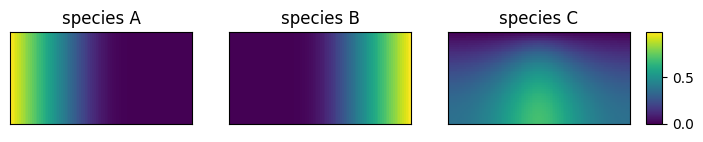
Position dependent Boundary Conditions
Boundary condition parameters can be arrays. For example, if c.shape=(n_x, n_y, n_c), then the coefficients for the boundary conditions in the x-direction (i.e., axis=0) can have the shape (1, n_y, n_c). This means at and , you can supply a value for each position and each component.
Until now, we supplied boundary conditions of the shape (1,1,n_c). Here, the direction is ‘singleton’. In the PyMRM implementations, these boundary conditions are ‘broadcasted’ along axis=1. This means the same value is used for every position.
As an example, let us consider the case where component is introduced on the left boundary through a hole between y_L_min and y_L_max, and is fed on the right between y_R_min and y_R_max. Component is removed on the upper boundary between x_U_min and x_U_max.
You can run the cell below to specify the position-dependent boundary conditions. Next, in the cell above, comment out the specification of the boundary conditions (so that the new ones are used) and rerun the cell.
# Define the inlet regions for boundary conditions
# Left boundary: A is introduced between y_L_min and y_L_max
y_L_min = 0.00 * L[1]
y_L_max = 0.50 * L[1]

# Right boundary: B is introduced between y_R_min and y_R_max
y_R_min = 0.50 * L[1]
y_R_max = 1.00 * L[1]

# Upper boundary: C is removed between x_U_min and x_U_max
x_U_min = 0.00 * L[0]
x_U_max = 0.25 * L[0]

# Helper function to create a filter for regions
def hole_filter(x, x_min, x_max):
    """Returns a boolean mask for positions within the specified range."""
    fltr = (x >= x_min) & (x < x_max)
    return fltr

# Initialize all positions on the left boundary as Neumann
a_L = np.ones((1,) + shape[1:])  # Coefficient for Neumann condition
b_L = np.zeros((1,) + shape[1:])  # Coefficient for Dirichlet condition
d_L = np.zeros((1,) + shape[1:])  # Dirichlet value

# Apply Dirichlet condition for A in the specified region on the left boundary
fltr = hole_filter(y_c, y_L_min, y_L_max)
a_L[:,fltr,0] = 0  # Switch to Dirichlet for A
b_L[:,fltr,0] = 1  # Set Dirichlet coefficient for A
d_L[:,fltr,0] = 1  # Set Dirichlet value for A
bc_L = {'a':a_L, 'b':b_L, 'd':d_L}

# Initialize all positions on the right boundary as Neumann
a_R = np.ones((1,) + shape[1:])  # Coefficient for Neumann condition
b_R = np.zeros((1,) + shape[1:])  # Coefficient for Dirichlet condition
d_R = np.zeros((1,) + shape[1:])  # Dirichlet value

# Apply Dirichlet condition for B in the specified region on the right boundary
fltr = hole_filter(y_c, y_R_min, y_R_max)
a_R[:,fltr,1] = 0  # Switch to Dirichlet for B
b_R[:,fltr,1] = 1  # Set Dirichlet coefficient for B
d_R[:,fltr,1] = 1  # Set Dirichlet value for B
bc_R = {'a':a_R, 'b':b_R, 'd':d_R}

# All positions on the bottom boundary are Neumann
bc_B = {'a':1, 'b':0, 'd':0}

# Initialize all positions on the upper boundary as Neumann
a_U = np.ones((shape[0], 1, shape[2]))
b_U = np.zeros((shape[0], 1, shape[2]))
d_U = np.zeros((shape[0], 1, shape[2]))

# Apply Dirichlet condition for C in the specified region on the upper boundary
fltr = hole_filter(x_c, x_U_min, x_U_max)
a_U[fltr,:,2] = 0  # Switch to Dirichlet for C
b_U[fltr,:,2] = 1  # Set Dirichlet coefficient for C
d_U[fltr,:,2] = 0  # Set Dirichlet value for C
bc_U = {'a':a_U, 'b':b_U, 'd':d_U}
Position Dependent Diffusion Coefficient
Diffusion coefficients can also be made position-dependent. However, it is important to note that diffusion coefficients are specified at the face positions of the grid. This means that you need to carefully use the appropriate grid variables (x_c, x_f, y_c, and y_f) when defining the coefficients.
Alternatively, you can define diffusion coefficients at cell centers and use PyMRM interpolation routines to obtain staggered values at the face positions.
As an example, consider a circular region within the domain where the diffusion coefficient is set to zero. This creates a no-diffusion zone. The code below demonstrates how to define such a region.
Important Notes:
For regions with zero diffusion, the stationary state depends on the initial state. For example, if components and are present, they will produce a certain amount of that cannot diffuse away. This means the steady state is not uniquely defined.
When using
dt=np.inf(steady-state assumption), the problem becomes singular because it lacks a unique solution. To address this, you can use a large but finite time step (dt) and initialize the domain with all concentrations set to zero. This ensures that the concentrations remain zero in the no-diffusion region.
To apply this, run the cell below to provide position dependent diffusion coefficients. Next, comment out the D_x_mat and D_y_mat in the 2D Diffusion Example, provide a large but finite time step dt, and rerun the example.
# Define the center and radius of the circular no-diffusion region
x_cntr = 0.5 * L[0]  # x-coordinate of the center
y_cntr = 0.5 * L[1]  # y-coordinate of the center
R = 0.3 * L[1]  # Radius of the circular region

# Function to create a mask for the circular region
def circle_mask(x, y, x_cntr, y_cntr, R):
    """Returns a boolean mask for positions outside the circular region."""
    return (x.reshape((-1, 1)) - x_cntr)**2 + (y.reshape((1, -1)) - y_cntr)**2 > R**2

# Apply the circular mask to the diffusion coefficients in the x-direction
D_x = circle_mask(x_f, y_c, x_cntr, y_cntr, R)[..., np.newaxis] * np.asarray(D).reshape((1, 1, -1))
D_x_mat = construct_coefficient_matrix(D_x)  # Construct the coefficient matrix for x-direction

# Apply the circular mask to the diffusion coefficients in the y-direction
D_y = circle_mask(x_c, y_f, x_cntr, y_cntr, R)[..., np.newaxis] * np.asarray(D).reshape((1, 1, -1))
D_y_mat = construct_coefficient_matrix(D_y)  # Construct the coefficient matrix for y-direction
Exercise
Play around with position dependent boundary conditions and diffusion coefficients.
Implement a position-dependent reaction rate constant, for example, only make a specific region reactive.
Implement composition dependent diffusion coefficients, e.g., using a Fick-Wilke mixing law.