Reactor Type: GLS Packed Bed (Trickle Bed) - Multiphase Reactor Modeling using PyMRM

Gas-liquid-solid (GLS) packed beds — commonly called trickle-bed reactors (TBRs) — have a gas and liquid flowing concurrently (downward) or counter-currently through a bed of catalyst pellets. They are ubiquitous in petroleum refining (hydrodesulfurization, hydrotreating), hydrogenation, and wastewater treatment. The trickle-flow regime features a gas-continuous phase with a liquid film over the catalyst.

Phase structure¶

Phase	Contents	Flow direction
Gas	H₂, light gases	Downward (co-current) or upward (counter-current)
Liquid	Heavy feed, solvents	Downward (trickle flow)
Solid catalyst	Active sites	Stationary

Flow regimes (Charpentier-Favier map):

Trickle flow: gas continuous, liquid trickles as films
Pulse flow: alternating liquid-rich and gas-rich pulses
Spray flow: liquid dispersed as droplets
Bubble flow: liquid continuous (high liquid rates)

Governing equations¶

Gas phase (plug flow, dissolved gas consumed):

v_G\frac{dc_G}{dz} = -k_G a_G (c_G - c_{Gi})

(1)

Liquid phase (dispersion + G-L transfer + L-S transfer + reaction):

v_L\frac{dc_L}{dz} = D_{ax,L}\frac{d^2 c_L}{dz^2} + k_L a_{GL}(c_{Li} - c_L) - k_{LS} a_{LS}(c_L - c_s)

(2)

Solid phase (pseudo-steady):

k_{LS} a_{LS}(c_L - c_s) = (1-\varepsilon)R(c_s)

(3)

Pressure drop (Larkins or Sai-Varma correlation for two-phase flow):

\left.\frac{\Delta P}{\Delta z}\right|_{TP} = \phi_L^2 \left.\frac{\Delta P}{\Delta z}\right|_{L,\text{single}}

(4)

where $\phi_L^2 = f(X_{LT})$ (Lockhart-Martinelli parameter).

PyMRM modeling strategy¶

Term	Implementation
Liquid convection	`construct_convflux_upwind` with $v_L$
Liquid dispersion	`construct_grad`, `construct_div` with $D_{ax,L}$
G-L mass transfer	Source: `kLa * (c_L_star - c_L)`
L-S mass transfer	Coupling: `kLS_aLS * (c_L - c_s)`
Solid reaction	`(1-eps)*R(c_s)` eliminates `c_s` analytically (1st order)
Henry’s law	`c_L_star = c_G / H` at G-L interface

import numpy as np
import matplotlib.pyplot as plt
import scipy.sparse as sp
import scipy.sparse.linalg as spla

# ── System parameters ─────────────────────────────────────────────
L, N = 2.0, 80
dz = L / N
z  = (np.arange(N) + 0.5) * dz

# Phase velocities (superficial)
v_G  = 0.05    # [m/s]
v_L  = 0.005   # [m/s]
eps  = 0.40    # total void fraction
eps_L = 0.15   # liquid holdup (Larkins correlation would give this)
eps_G = eps - eps_L

# Mass-transfer parameters
kLa_GL  = 0.05     # gas-liquid volumetric kL [1/s]
kLS_aLS = 0.5      # liquid-solid volumetric kLS [1/s]
H_inv   = 30.0     # 1/Henry = c_L*/c_G (solubility)
k_s     = 1.0      # solid reaction rate [1/s]
Dax_L   = 5e-4     # liquid axial dispersion [m²/s]

# Inlet conditions
c_G_in = 1.0   # gas concentration at inlet [mol/m³]
c_L_in = 0.0   # liquid concentration at inlet

# ── Gas phase (plug flow, simple ODE solved as 1D linear system) ───
# v_G dc_G/dz = -kLa_GL*(c_G - c_Li) approximately with c_Li ~ c_L/H_inv
# For simplicity: assume gas plug-flow, liquid controls resistance
# Gas depletion: v_G dc_G/dz + kLa_GL*c_G = kLa_GL*c_L_prev/H_inv
# Solve iteratively: start with c_L = 0, update gas, update liquid

c_G = np.ones(N) * c_G_in
c_L = np.zeros(N)

# Build liquid-phase matrix (constant for given c_G)
# -Dax dc_L/dz + v_L dc_L/dz - kLa_GL*(c_G/H_inv - c_L) + kLS_aLS*(c_L - c_s) = 0
# c_s = kLS_aLS * c_L / (kLS_aLS + (1-eps)*k_s)   [pseudo-steady solid]
alpha_s = kLS_aLS / (kLS_aLS + (1-eps)*k_s)
k_eff_L = kLS_aLS * (1 - alpha_s)  # effective liquid sink

off_L   = Dax_L / dz**2
A_L     = sp.diags([-off_L - v_L/dz,
                     2*off_L + v_L/dz + kLa_GL + k_eff_L,
                    -off_L],
                   [-1, 0, 1], shape=(N, N), format='csr')
# BC: Danckwerts at inlet
A_L     = A_L.tolil()
A_L[0,0] -= off_L
A_L = sp.csr_matrix(A_L)

# Build gas matrix (plug flow)
A_G = sp.diags([-v_G/dz, v_G/dz + kLa_GL/H_inv],
               [-1, 0], shape=(N, N), format='csr')

# Iterative G-L coupling
for iteration in range(20):
    # Gas: source = kLa_GL * c_L * H_inv
    rhs_G = kLa_GL / H_inv * c_L
    rhs_G[0] += v_G/dz * c_G_in
    c_G_new = spla.spsolve(A_G, rhs_G)
    # Liquid: source = kLa_GL * c_G / H_inv
    rhs_L = kLa_GL / H_inv * c_G_new
    rhs_L[0] += (off_L + v_L/dz) * c_L_in
    c_L_new = spla.spsolve(A_L, rhs_L)
    res = np.max(np.abs(c_L_new - c_L)) + np.max(np.abs(c_G_new - c_G))
    c_G, c_L = c_G_new, c_L_new
    if res < 1e-10: break

c_s = alpha_s * c_L

plt.figure(figsize=(7, 4))
plt.plot(z, c_G, 'b-', label='Gas c_G')
plt.plot(z, c_L / H_inv, 'g--', label='c_L / H (liquid, scaled)')
plt.plot(z, c_s / H_inv, 'r:', label='c_s / H (solid)')
plt.xlabel('z (m)'); plt.ylabel('Concentration (scaled)')
plt.title('Trickle-bed reactor: G-L-S profiles')
plt.legend(); plt.tight_layout(); plt.show()
X_G = 1 - c_G[-1] / c_G_in
print(f'Gas conversion: {X_G*100:.1f}%')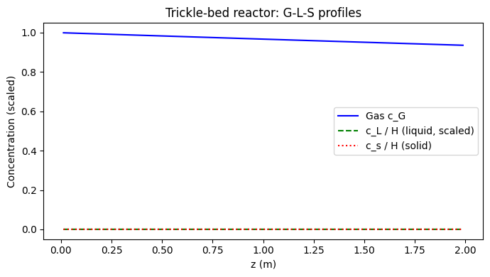

Gas conversion: 6.4%

Summary¶

Trickle-bed reactors combine gas-liquid mass transfer with liquid-solid mass transfer and reaction
Three resistances in series: G-L ( $1/k_G a$ ), L-S ( $1/k_{LS} a_{LS}$ ), internal particle ( $1/\eta k$ )
The limiting resistance determines which correlation is most critical for design
Liquid holdup from Larkins or Sai-Varma correlation sets available liquid-solid contact area
Iterative G-L coupling converges quickly when resistances are not too different in magnitude